- Stability analyses for flexural buckling, torsional buckling, and flexural-torsional buckling under compression
- Import of the effective lengths from the calculation using the Structure Stability add-on
- Graphical input and check of the defined nodal supports and effective lengths for stability analysis
- Determination of the equivalent member lengths for tapered members
- Consideration of Lateral-Torsional Bracing Position
- Lateral-torsional buckling analysis of the structural components subjected to moment loading
- Depending on the standard, a choice between user-defined input of Mcr, analytical method from the standard, and use of internal eigenvalue solver
- Consideration of a shear panel and a rotational restraint when using the eigenvalue solver
- Graphical display of a mode shape if the eigenvalue solver was used
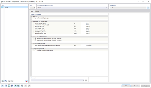
- Stability analysis of structural components with the combined compression and bending stress, depending on the design standard
- Comprehensible calculation of all necessary coefficients, such as the factors for considering moment distribution or interaction factors
- Alternative consideration of all effects for the stability analysis when determining internal forces in RFEM/RSTAB (second-order analysis, imperfections, stiffness reduction, possibly in combination with the Torsional Warping (7 DOF) add-on)
You can enter the structural system and calculate the internal forces in the programs RFEM and RSTAB. You have full access to the extensive material and cross-section libraries.
Timber Design is completely integrated into the main programs. At the same time, it automatically takes into account the structure and the available calculation results. You can assign further entries for the timber design, such as effective lengths, cross-section reductions, or design parameters, to the objects to be designed. You can easily select the elements graphically using the [Select] function at many places of the program.
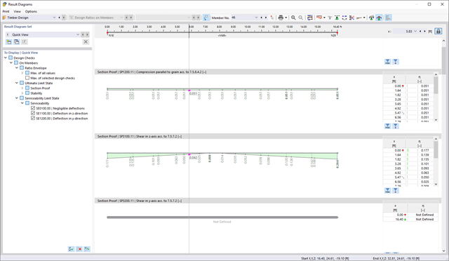
If your design is successful, the relaxed part of your work follows. Because the program does many processes for you. For example, the performed design checks are displayed in a table. It shows you all the result details. Due to the clearly presented design formulas, you will be able to understand the results without any problems. There is no "black box" effect here.
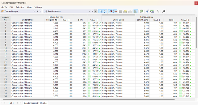
The design checks are carried out at all governing locations of the members and displayed graphically as a result diagram. Furthermore, detailed graphics, such as the stress distribution on a cross-section or the governing mode shape, are available for you in the result output.
All input and result data are part of the RFEM/RSTAB printout report. You can select the report contents and extent specifically for the individual design checks.
For joint components, you can check whether the stability failure is relevant. This requires the Structure Stability add-on for RFEM 6.
In this case, you calculate the critical load factor for all analyzed load combinations and the selected number of mode shapes for the connection model. Compare the smallest critical load factor with the limit value 15 from the standard EN 1993‑1‑1, Clause 5. Furthermore, you can make user-defined adjustment of the limit value. As a result of the stability analysis, the program displays the corresponding mode shapes graphically.
For the stability analysis, RFEM uses the adapted surface model to specifically recognize the local buckling shapes. You can also save and use the model of the stability analysis, including the results, as a separate model file.
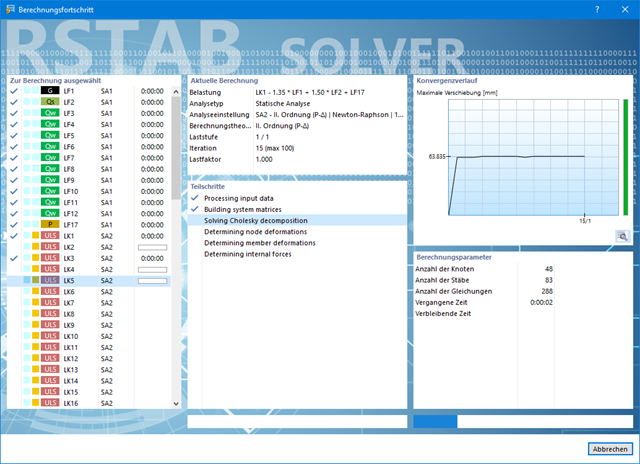
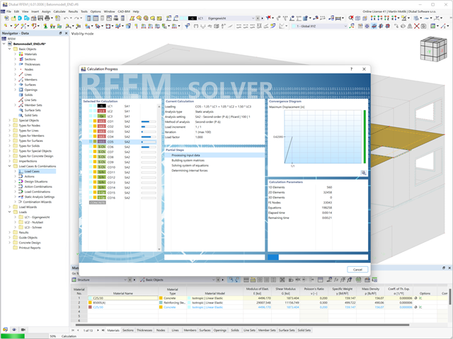
Also in this case, RSTAB will certainly convince you. With the powerful calculation kernel, its optimized networking and support of multi-core processor technology, the Dlubal structural analysis program is far ahead. This allows you to calculate more linear load cases and load combinations using several processors in parallel without using additional memory. The stiffness matrix only has to be created once. Thus, it is possible for you to calculate even large systems with the fast and direct solver.
Do you have to calculate multiple load combinations in your models? The program initiates several solvers in parallel (one per core). Each solver then calculates a load combination for you. This leads to better utilization of the cores.
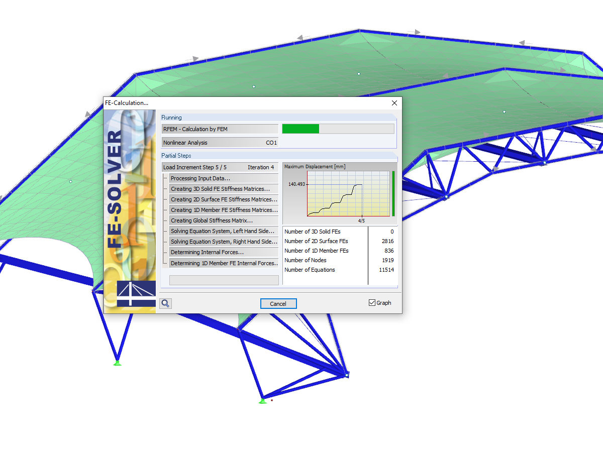
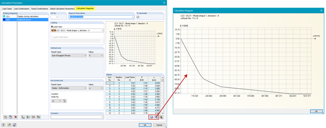
You can systematically follow the development of the deformation displayed in a diagram during the calculation, and thus precisely evaluate the convergence behavior.

Do you know exactly how the form-finding is performed? First, the form-finding process of the load cases with the load case category "Prestress" shifts the initial mesh geometry to an optimally balanced position by means of iterative calculation loops. For this task, the program uses the Updated Reference Strategy (URS) method by Prof. Bletzinger and Prof. Ramm. This technology is characterized by equilibrium shapes that, after the calculation, comply almost exactly with the initially specified form-finding boundary conditions (sag, force, and prestress).
In addition to the pure description of the expected forces or sags on the elements to be formed, the integral approach of the URS also enables a consideration of regular forces. In the overall process, this allows, for example, for a description of the self-weight or a pneumatic pressure by means of corresponding element loads.
All these options give the calculation kernel the potential to calculate anticlastic and synclastic forms that are in an equilibrium of forces for planar or rotationally symmetric geometries. In order to be able to realistically implement both types individually or together in one environment, the calculation provide you with two ways to describe the form-finding force vectors:
- Tension method - description of the form-finding force vectors in space for planar geometries
- Projection method - description of the form-finding force vectors on a projection plane with fixation of the horizontal position for conical geometries

Did you know that Equivalent static loads are generated separately for each relevant eigenvalue and excitation direction. These loads are saved in a load case of the Response Spectrum Analysis type and RFEM/RSTAB performs a linear static analysis.
The program supports you: It determines the bolt forces on the basis of the FE analysis model and evaluates them automatically. The add-on performs the standard-compliant design of bolt resistance for failure cases, such as tension, shear, hole bearing, and punching, and clearly displays all required coefficients.
Do you want to perform weld design? The welds are modeled as elastic-plastic surface elements, and their stresses are read out from the FE analysis model. The plasticity criteria is set in the way that they represent failure according to AISC J2-4, J2-5 (strength of welds), and J2-2 (strength of base metal). The design can be performed with the partial safety factors of the selected National Annex of EN 1993‑1‑8.
The plates in the connection are designed plastically by comparing the existing plastic strain to the allowable plastic strain. The default setting is 5% according to EN 1993‑1‑5, Annex C, but can be adjusted by user-defined specifications, as well as 5% for AISC 360.

In RFEM, you can use these three powerful eigenvalue solvers:
- Root of Characteristic Polynomial
- Method by Lanczos
- Subspace Iteration
RSTAB, on the other hand, provides you with these two eigenvalue solvers:
- Subspace Iteration
- Shifted inverse power method
The selection of the eigenvalue solver depends primarily on your model size.
- Free definition of two reinforcement layers
- Design alternatives to avoid compression or shear reinforcement
- Design of surfaces as deep beams (theory of membranes)
- Option to define basic reinforcements for top and bottom reinforcement layers
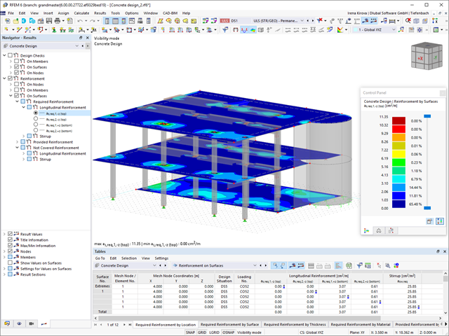
- Free definition of provided surface reinforcement
- Result output in points of any selected grid
- Design with design moments at column edges
- Determination of deformation in state II; for example, according to EN 1992‑1‑1, 7.4.3, and ACI 318‑19 24.2.3, Table 24.2.3.5
- Considering tension stiffening
- Considering creep and shrinkage
- Fatigue design according to EN 1992‑1‑1, Chapter 6.8 (see this Product Feature)
- Design of a shear joint between the web and flange of ribs
- Optional pure slab or wall design of surfaces for a 2D model type
- Precise breakdown of reasons for failed design
- Design details of all design locations for better traceability of reinforcement determination
You have two options in RFEM. On the one hand, you can determine the punching load from a single load (from column/loading/nodal support) and the smoothed or unsmoothed shear force distribution along the control perimeter. On the other hand, you can specify them as user-defined.
Calculate the design ratio of the punching shear resistance without punching reinforcement as a design criterion and the program will deliver you the corresponding result. In the case of exceeding the punching shear resistance without punching reinforcement, the program determines the required punching reinforcement as well as the required longitudinal reinforcement for you.

If there are geometry differences arising between the ideal and the deformed structural system from the previous construction stage, they are compared in the program. The next construction stage is built on top of the stressed system from the previous construction stage. This calculation is nonlinear.
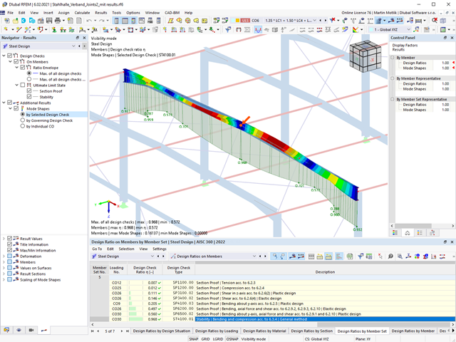
- Stability analyses for flexural buckling, torsional buckling, and flexural-torsional buckling under compression
- Import of the effective lengths from the calculation using the Structure Stability add-on
- Graphical input and check of the defined nodal supports and effective lengths for stability analysis
- Lateral-torsional buckling analysis of the structural components subjected to moment loading
- Depending on the standard, a choice between user-defined input of Mcr, analytical method from the standard, and use of internal eigenvalue solver
- Consideration of a shear panel and a rotational restraint when using the eigenvalue solver
- Graphical display of a mode shape if the eigenvalue solver was used
- Stability analysis of structural components with the combined compression and bending stress, depending on the design standard
- Comprehensible calculation of all necessary coefficients, such as the factors for considering moment distribution or interaction factors
- Alternative consideration of all effects for the stability analysis when determining internal forces in RFEM/RSTAB (second-order analysis, imperfections, stiffness reduction, possibly in combination with the Torsional Warping (7 DOF) add-on)
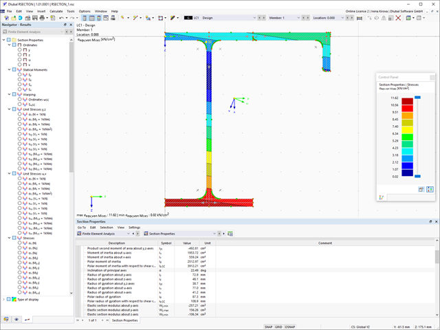
RSECTION calculates all relevant cross-section properties. This also includes the plastic limit internal forces. In the case of cross-sections consisting of different materials, RSECTION determines the ideal cross-section properties.
You have various options with RSECTION. For example, you can calculate the stresses from axial force, biaxial bending moments and shear forces, primary and secondary torsional moment, and warping bimoment for any cross-section shape. Determine the equivalent stresses according to the stress hypothesis by von Mises, Tresca, and Rankine.
Convince yourself by the powerful calculation kernel, its optimized networking and support of multi-core processor technology. This provides you with the advantages, such as parallel calculations of linear load cases and load combinations using several processors without additional demands on the RAM. The stiffness matrix only has to be created once. Thus, you can calculate even large systems with the fast direct solver.
If you need to calculate multiple load combinations in your models, the program initiates several solvers in parallel (one per core). Each solver then calculates a load combination, which improves the core utilization.
You can systematically follow the development of the deformation displayed in a diagram during the calculation, and thus precisely evaluate the convergence behavior.
Select the individually suitable calculation parameters for your project: You can perform the calculation for all member types according to the linear static, second-order, or large deformation analysis. You have this selection option for load cases and load combinations. You can specifically set further calculation parameters for load cases, load combinations, and result combinations, which ensures a high degree of flexibility with regard to the calculation method and detailed specifications.
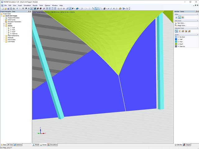
In RWIND Simulation, it is possible to divide the model in different zones. This allows for different surface roughness to be assigned to the zones. In addition, local results can be better evaluated.
.png?mw=640&hash=9aa98962d5e0d0ed2803b35fcb6a2f87288b0946)
The number of degrees of freedom in a node is no longer a global calculation parameter in RFEM (6 degrees of freedom for each mesh node in 3D models, 7 degrees of freedom for the warping torsion analysis). Thus, each node is generally considered with a different number of degrees of freedom, which leads to a variable number of equations in the calculation.
This modification speeds up the calculation, especially for models where a significant reduction of the system could be achieved (for example, trusses and membrane structures).
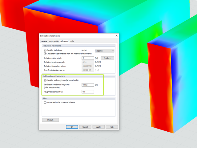
Utilize the RWIND Simulation program to consider a surface roughness of the model surface by applying a modified wall boundary condition. The numerical model is based on the assumption that grains with a certain diameter are arranged homogeneously on the model surface, similar to sandpaper. The grain diameter is described with the parameter Ks and the distribution with the parameter Cs. By considering the wall roughness, the numerical flow simulation can capture reality more closely.
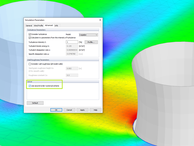
The volume space in RWIND Simulation can optionally be discretized with the second-order theory between the cells.
This extended approach usually results in more accurate results despite poorer convergence behavior.
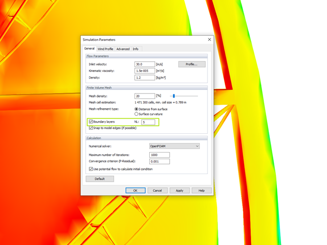
The meshing algorithm of RWIND Simulation uses the boundary layer option to mesh the area near the model surface with a voluminous layer mesh. The number of layers is controlled by a user-defined parameter.
This fine mesh in the area of the model surface helps to represent the wind velocity close to the surface.
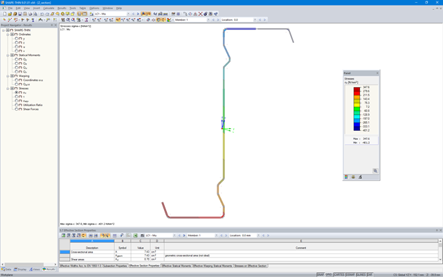
SHAPE‑THIN determines the effective cross-sections according to EN 1993‑1‑3 and EN 1993‑1‑5 for cold-formed sections. You can optionally check the geometric conditions for the applicability of the standard specified in EN 1993‑1‑3, Section 5.2.
The effects of local plate buckling are considered according to the method of reduced widths, and the possible buckling of stiffeners (instability) is considered for stiffened sections according to EN 1993‑1‑3, Section 5.5.
As an option, you can perform an iterative calculation to optimize the effective cross-section.
You can display the effective cross-sections graphically.
Read more about designing cold-formed sections with SHAPE-THIN and RF-/STEEL Cold-Formed Sections in the technical article "Design of Thin-Walled, Cold-Formed C-Section According to EN 1993‑1‑3".
Design of Thin-Walled, Cold-Formed C-Section According to EN 1993-1-3 More about RF-/STEEL Cold-Formed Sections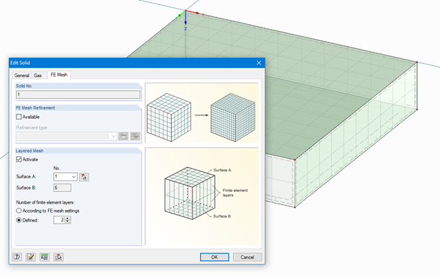
The stiffness of gas given by the ideal gas law pV = nRT can be considered in the nonlinear dynamic analysis.
The calculation of gas is available for accelerograms and time diagrams for both the explicit analysis and the nonlinear implicit Newmark analysis. To determine the gas behavior correctly, at least two FE layers for gas solids should be defined.
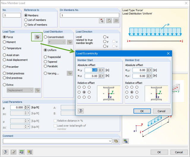
You can define eccentricities for member loads of the load type 'Force'. You can apply the load eccentricities by means of an absolute or relative offset.
We recommend using the large deformation analysis to consider all effects of eccentric loads.

You can create various load cases with a single mouse click. After the generation, the numbers of created load cases and result combinations are displayed.

In SHAPE-THIN 8, the effective cross-section of stiffened buckling panels can be calculated according to EN 1993-1-5, Cl. 4.5.
The critical buckling stress is calculated according to EN 1993-1-5, Annex A.1 for buckling panels with at least 3 longitudinal stiffeners, or according to EN 1993-1-5, Annex A.2 for buckling panels with one or two stiffeners in the compression zone. The design for torsional buckling safety is also performed.
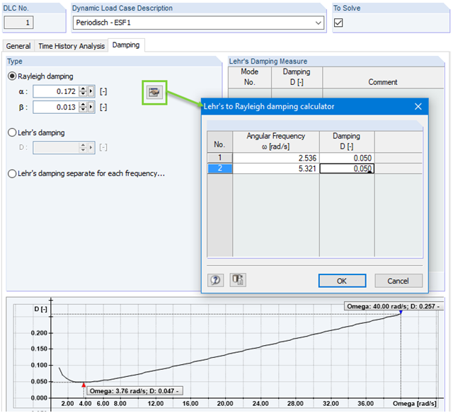
Calculation with consideration of a damping ratio (or Lehr's damping) is not possible in the direct time step integrations. Instead, the Rayleigh damping coefficients must be specified by the user.
In technical literature, the given damping ratio for specific construction forms is, in many cases, only a rough approximation of the real damping ratios. In RF-/DYNAM Pro - Forced Vibrations, it is possible to use the value of the damping ratio to determine the Rayleigh damping. This may occur at one or two natural angular frequencies defined by the user.

If the check box 'Number of load increments' is deactivated, the number of load increments will be determined automatically in RFEM to solve nonlinear tasks efficiently.
The method used is based on a heuristic algorithm.
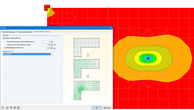
With this function, it is possible to refine the FE mesh on surfaces automatically. The mesh refinement is gradual. In each step, the FE mesh is recreated based on an error comparison of the results in the previous calculation step. The numerical error is evaluated from the results of surface elements and is based on the energy formulation of Zienkiewicz-Zhu.
The error evaluation is carried out for a linear static analysis. We select a load case (or load combination) for which the FE mesh is generated. The FE mesh is then used for all calculations.
In RFEM, it is possible to determine pushover curves (also called capacity curves) and export them to Excel.
With the RF-DYNAM Pro - Equivalent Loads add-on module, it is possible to generate load distribution automatically in accordance with a mode shape and export it as a load case to RFEM.