The results can also be checked in the tables.
The 'Static Analysis' tables were set automatically after the calculation. In the list next to it in the table toolbar, the model objects can be selected to display the results by nodes, lines, members, or surfaces.
Node Results
To see the support forces table for the column footings, select Results by Node from the list (1). The nodal results are managed by two different tables. Click the Support Forces tab (2).
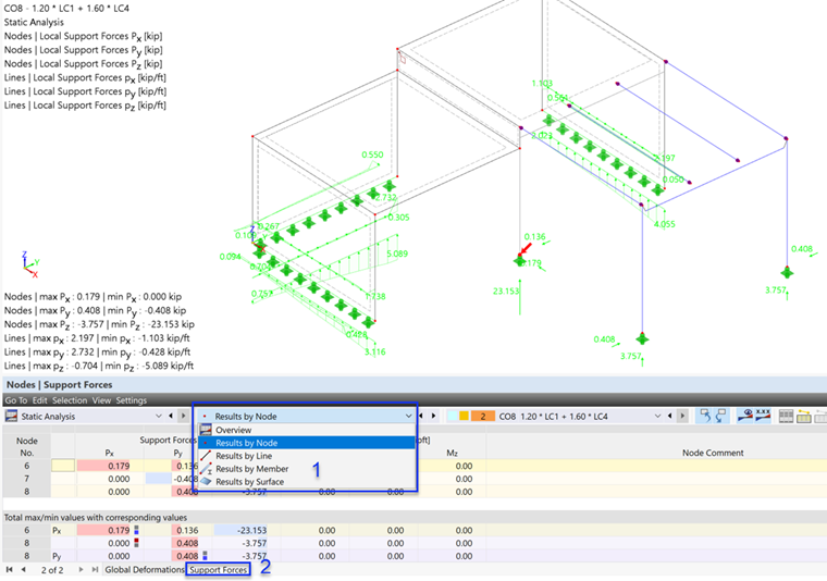
The upper part of the table shows the results for each of the three supported nodes. In the lower part, the maximum and minimum values with regard to the local directions of the supports are listed (in this tutorial, the latter coincide with the global directions).
The object of the selected table line is marked by an arrow in the graphics so that you can easily locate it.
Surface Results
To check the stresses of the surfaces in the table, select Results by Surface from the toolbar list (1). Then click the Basic Stresses tab (2). The axial stresses and shear stresses are listed for every 'Grid Point' of each surface.
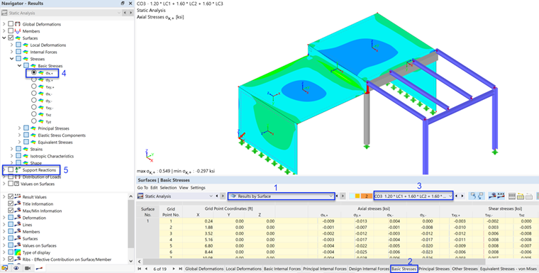
Set CO3 in the table toolbar to display the stresses due to the live loads on both slabs (3). To view the stresses in the graphics, too, open the Basic Stresses item of the Stresses subcategory and select σx,+, for example (4). Those stresses represent the axial stresses in the local x-direction of each surface. The "+" symbol signifies the positive side of the surface which is in direction of its local z-axis – the bottom side of each slab, for example.
For a better view of the surface stresses, switch off the Support Reactions (5).
There are singularity effects around the concrete column. They can be explained by the load flow from the surfaces to a member via a single node.
To display the results in the grid points in the graphics, too, select the Values on Surfaces option in the upper part of the navigator.
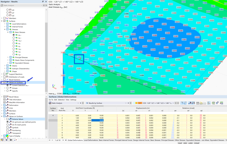
Again, the grid point of the current line is marked by an arrow in the graphics.
Adjusting the Grid
As you can see by the coordinates in the table, a grid of 1.0 ft defined by default. It can be adjusted for every surface, if necessary: Double-click a surface, for example no. 4 or no. 5, by its dashed lines (see the ‘Symbol of surfaces’ image) to open the 'Edit Surface' dialog box. Select the Grid tab.
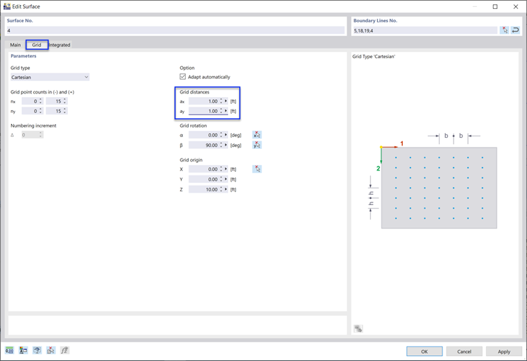
The 'Grid distances' control the number of grid points to be created in the x- and y-directions of the surface. In our example, 1.0 ft grid distances are suitable. Click OK.