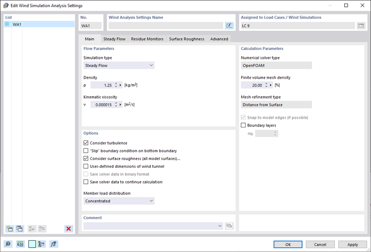
You can define the general flow parameters on the Main tab.
Flow Parameters
This area controls the simulation type. You can choose between two types of the simulation.
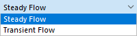
In Chapters Steady Flow and Transient Flow (non-stationary flow), the specific settings are described for each simulation type and the corresponding tabs.
The "Density" of the air is dependent on the altitude, temperature, atmospheric pressure and humidity. It has an effect on the dynamic behaviour of the fluid.
The value of the "Kinematic viscosity" describes the resistance of the air to deformation. It is defined as the ratio of the viscosity to the density of the air.
Options
For calculation with RWIND 2, the effects of turbulence are essential. If you want to "Consider turbulence," activate the check box. The effects of turbulent flow are characterized by chaotic changes of pressure and flow velocity, contrasting laminar flow. For further explanation, see Chapter Turbulence.
The slip boundary condition applied to the bottom surface of the wind tunnel can be set by activating the "Slip boundary condition on bottom boundary" check box. For more about boundary conditions, see Chapter Wind Tunnel.
When the "Consider surface roughness" check box is activated, the roughness is taken into account for every surface of the model (see Chapter Advanced). You can define the roughness parameters on the Surface Roughness tab.
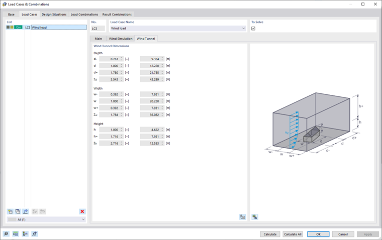
The "User-defined dimensions of wind tunnel" check box enables you to define the tunnel size manually. For more details on the tunnel parameters, see Chapter Wind Tunnel. You can then define the tunnel dimensions on the "Wind Tunnel" tab of the "Load Cases & Combinations" dialog box.
The "Save solver data to continue calculation" check box allows you to continue the calculation even after the project is closed and reopened (see Chapter Steady Flow ).
Member Load Distribution
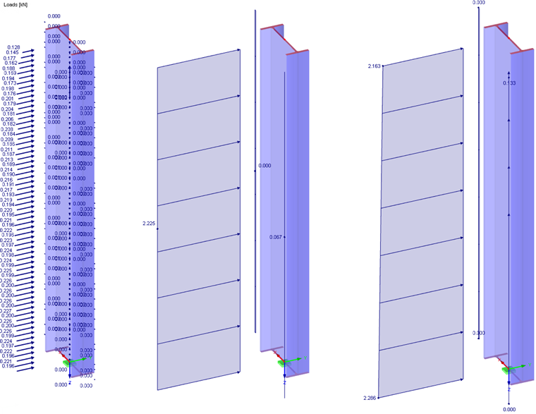
The setting has an effect on the load application of the generated member loads on the model.
- Concentrated: The loads result in concentrated loads at relative distances along every member. The intervals of the load application points are usually very small, depending on the density of the mesh.
- Uniform: For every member, constant loads are created along the member length. Only one uniform member load is applied for each global direction.
- Trapezoidal: Similar to uniform loads, the concentrated loads are levelled along the member. They are converted into a trapezoidal distribution, however, to approximate the actual gradients.
Calculation Parameters
The "Numerical solver type" is the current CFD Solver used by RWIND 2. It is the external CFD code OpenFOAM®. More information is available in Chapter CFD Solver.
The finite volume density of mesh to be applied around the model is controlled by percentage reference. This specific refinement is utilized for the model simplification and the flow calculation. The default density (20%) normally results in a relatively low number of finite volumes and a relatively fast calculation. The minimum percentage is 10%. It entails a rather coarse mesh with the smallest number of volumes. The higher the density of the mesh, the smaller the size of the finite volume cells will be. The results are accordingly more precise, but the calculation will need more time due to the greater number of volumes. Setting the maximum mesh density (100%) leads to very fine meshes with millions of volumes. The calculation of 3D flow on such meshes is on the edge of the capabilities of current PCs, with a calculation time of several hours to several days.
For further information, see Chapter Computational Mesh and Model Simplification.
The "Mesh refinement type" can be defined for curvatures of the model surfaces or globally for a distance from the model surfaces, see Chapter General, Finite Volume Mesh.
The "Boundary layers" option controls whether the finite volume mesh next to the surfaces of the model is refined in a special way. This refinement gives better results near the boundaries of the model (see the image
Finite Volume Mesh with Five Boundary Layers
). We highly recommend activating the boundary layers and defining the number of layers NL when the surface roughness is to be taken into
account.