The steady flow calculation can be selected on the "General" tab of the "Simulation Parameters" dialog box (see the image
Simulation Parameters
).
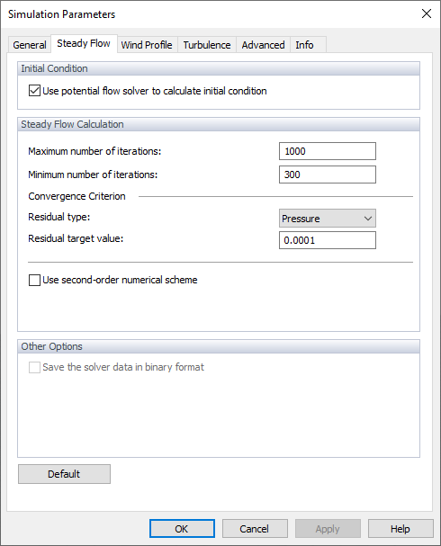
Initial Conditions
When activating the "Use potential flow to calculate the initial condition" option, a linearized version of the non-viscous Navier‑Stokes equations is used to generate the start conditions.
Steady Flow Calculation
You can define the "Maximum number of iterations." By default, the limit is 500 iterations. If the calculation converges within fewer iterations, it is stopped. You can also define "Minimum number of iterations", which is set to 300 iterations by default (see the image
Program Options
), regardless of whether the convergence criterion (see below) has already been met. The maximum number is useful to avoid infinite loops.
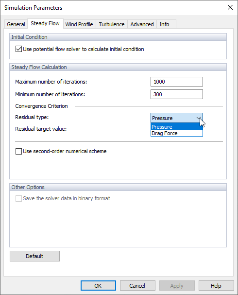
The "Convergence criterion" represents the stop limit for the calculation. There are two convergence criteria available, you can follow the pressure criterion or the drag force criterion. Select one of the options in the Residual Type and then set the target value.
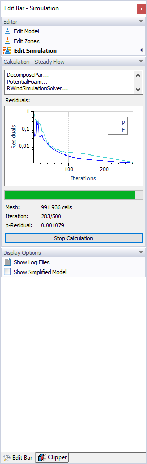
As soon as the residual quantity falls below the defined value, the calculation is terminated. The diagram of iterations and residual quantity (p-Residual for pressure) is shown during the calculation. It is also available in the simulation results (see Chapter Residuals).
The "Use second-order numerical scheme" check box controls which numerical scheme is used for divergence terms (fluxes). It is not activated by default, so the calculation is carried out according to the first order. If the check box has been selected, the solution is performed according to the second order.
Other Options
The steady-state solver of RWIND 2 does not fully capture the "oscillating" effects as described in FAQ 4731. In order to solve the partial differential equations numerically, all differential terms (space and time derivatives) have to be discretized. You can find more information about solvers in the Algorithms and Solvers documentation. There is a vast list of discretizations ("schemes"), with each scheme having a particular numerical behaviour in view of accuracy, stability, and convergence. For more information about the convergence, see CFD Direct.