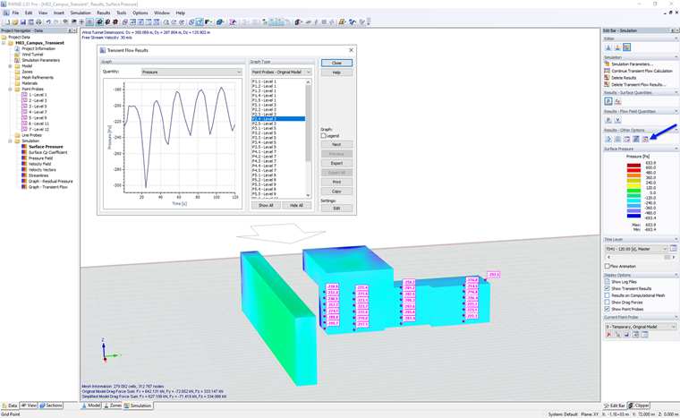
These graphs show the time development of quantities (pressure, velocity and Cp coefficient) at the points of the given probe. The probes are divided into three groups according to the type of mesh on which its points are located: A "Flow Field" mesh, an "Original model" mesh, and a "Simplified model" mesh; for more about the probes, see Chapter Probes.
The exceptions are "Point Probes" on the "Original Model," whose curves are always plotted from transient-flow data for the entire domain. This is due to technical reasons associated with extrapolating the pressure on the original model. The curves lying on the original model have another peculiarity, namely the case where the original model consists in a flat plate that has two different result values at one point (for example, different pressure on the front and back sides of the plate). In such cases, two different curves are plotted in the graph and are marked with a special suffix: "Front" and "Back", see Mesh Section in Chapter Sections.
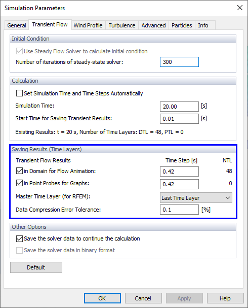
To summarize, before the calculation it is necessary to define the Point Probes in the place of interest and activate data saving for graphs in the Simulation Parameters dialog box, then after the transient calculation you can display the curves for the selected point probe in the given time layer, as you can see in the image below.
The names of curves in the graph correspond to the numbering of the probe points, which can be displayed in the graphics according to the image below.