Turbulence is one of the most complicated phenomena observed in nature, making a precise definition difficult. In turbulent flow, the fluid follows irregular curved paths called eddies. Generally, the flow is intertwined and creates structures of many different sizes. They move and rotate instantaneously, interact with each other and the main flow field and they change shape and size rapidly. The mixing is significant and affects momentum diffusion and, as consequence, the aerodynamic forces within a fluid and surrounding obstacle, such as buildings. If you want to study this complicated phenomenon and look under the bonnet, we recommend this Introduction to Turbulence. [1]
The turbulent structures cause in the fluid the vorticity, which is often used to describe turbulence rather than velocity.
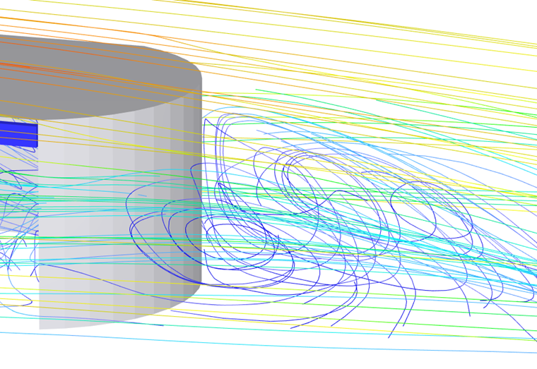
Vorticity is primarily generated at solid boundaries. In the boundary layers formed along solid boundaries, the velocity varies from zero at the boundary (no-slip condition) to a value mostly unaffected by the boundary, determined by the flow. Turbulence occurs, when instabilities, such as roughness of the boundary surface, cause the vorticity to become chaotic, sustained by a sufficiently high Reynolds number. The boundary layer breaks away from the boundary, vorticity and turbulence are thereby swept into regions of fluid away from the boundaries. Large eddies are usually anisotropic (for example flow past a cylinder causes shedding of vortices). Flow disturbances trigger instabilities which cause vortices to stretch, compress and disappear. Coherent flow structures rapidly disintegrate into a mass of turbulent eddies with growth of isotropy on large scale. Large eddies become smaller until they reach a size where the dissipation of their kinetic energy due to viscosity is significant. The loss of kinetic energy causes these eddies to vanish. [3]
For an incompressible fluid the vorticity obeys the transport equation.
Numerical Modelling of Turbulence
In order to fully capture turbulence by numerical modelling, the equations of motion for fluid flow on all spatial and temporal scales must be solved. There does not exist one suitable universal method.
The exact method calculating the flow using the above-mentioned equations for all scales, referred to as "Direct Numerical Simulation" (DNS), is not applicable for practical CFD due to its computational costs. The computational resources required by DNS far exceed the capacity of the most powerful supercomputers currently available.
"Large-Eddy Simulation" (LES) instead uses accurate numerical schemes such as DNS for large scales, while for the small scales modelling of turbulence is used (so called subgrid-scale modelling). It has severe limitations in the near wall regions, as the computational effort required for the boundary layer, where turbulence length scale becomes very small, grows rapidly. However, for free shear flows, where the large eddies are at the order of magnitude as the shear layer and strongly anisotropic, LES may provide extremely reliable results. It is useful to resolve problems such as flow induces vibrations etc.
For most practical CFD problems the computational costs of DNS and to a lesser extent LES is too great. Instead, "Reynolds-Averaged Navier-Stokes" (RANS) equations method is much more affordable (see subchapter RANS Models for Turbulence.
For more complex problems, where advantages of the above-mentioned methods are required, but the computational costs must remain reasonable, so-called "Global hybrid methods" can be used (see subchapter Global Hybrid Models for Turbulence). The Global hybrid methods are based on combination of LES and RANS methods switching them as the resolution level changes. RANS is applied for a portion of the boundary layer and large eddies are resolved away from these regions by LES. The most popular models are "Detached Eddy Simulation" (DES) or "Delayed Detached Eddy Simulation" (DDES).
RANS Models for Turbulence
For steady flows, RWIND 2 uses Reynolds-Averaged Navier-Stokes Equations (RANS) model of turbulence. RANS is based on the Reynolds decomposition according to which a flow variable is decomposed into mean and fluctuating components. When the decomposition is applied to Navier-Stokes equations, an extra term known as the "Reynolds Stress Tensor" arises and a system of equations needs to be “closed”. Levels of RANS turbulence models are related to the number of differential equations added to RANS equations in order to “close” them. [2]
The most popular two-equation models k-ε a k-ω are available also in RWIND 2. One-equation “Spalart-Allmaras” (SA) turbulence model has been developed specifically for aerodynamic flows and is also used often in the Global hybrid methods. It is used in RWINDS 2 Pro for modelling turbulence in transient flows (see subchapter [#GlobalHybridModelsForTurbulence Global hybrid models for turbulence])
k-ε Turbulence Model
The k-ε model was the first turbulence model to be widely used for a variety of flows in CFD. It is based on analogy of the random motion of eddies in a turbulent fluid flow with particles at a molecular scale, suggested by Boussinesq. He introduced the concept of eddy viscosity, which is not fluid property but is proportional to a characteristic speed and length scale of the turbulence. The models are required to represent each of these scales. The speed scale is represented by turbulent kinetic energy k, described by a transport equation. The k-equation includes a term for its rate of dissipation ε; a transport equation for ε, provides a model for that term – which also represents the length scale of turbulence. [2], [3]
The k- ε model is robust and computationally cheap. It is valid for fully turbulent flows only. Therefore, it is suitable for initial iterations and parametric studies. It performs poorly for complex flows involving severe or adverse pressure gradient, separations and strong streamline curvatures. It also behaves troublesome at boundaries.
k-ω Turbulence Model
The k-ω model “closes” the RANS system by two partial differential equations for k and ω, with the first variable being again the turbulence kinetic energy and the second being the specific rate of dissipation (of the turbulence kinetic energy k into internal thermal energy). Its better dissipation term gives the k- ω model an advantage over k- ε model in the near-wall region. It has also good performance for free shear and low Reynolds number flows. It is more suitable for complex boundary layer flows and separation in external aerodynamics (however, the flow separation is typically predicted too excessive and early, and therefore requires high mesh resolution near the wall). It can be used also for transitional flows.
Two-equation models contain many assumptions and are calibrated to work well only according to well-known features of the applications they are designed to solve. Nonetheless, their strength has proven itself and the industry CFD calculations use them widely.
Global Hybrid Models for Turbulence
The idea of the global hybrid models is to benefit from advantages of the available RANS and LES models. The RANS method is applied for a portion of the boundary layer, where LES would have high computational costs, and the rest of the flow with large eddies is resolved by LES, where RANS cannot model well anisotropic turbulent structures. In other words, regions where the turbulent length scale is less than the maximum grid dimension are assigned the RANS mode of solution. As the turbulent length scale exceeds the grid dimension, the regions are solved using the LES mode, thereby cutting the computational costs significantly yet still offering some of the advantages of the LES method in separated regions.
Spalart-Allmaras DDES Model
In transient flow analysis (only in RWIND 2 Pro), a global hybrid model “Spalart-Allmaras Delayed Detached Eddy Simulation” is used, see Openfoam®.
The main improvement of the "Delayed Detached Eddy Simulation" (DDES) is to include the turbulent viscosity information into the switching mechanism to delay this switching in boundary layers. The RANS system is “closed” by one eddy-viscosity transport equation according to "Spalart-Allmaras model" with incorporated model length scale to the wall distance.
Spalart-Allmaras single-equation turbulent model that solves the modeled transport equation for the eddy turbulent viscosity νT. The equation resolves a Spalart-Allmaras, viscosity-like variable ṽ. Simply put, the variable ṽ is easier to calculate than νT directly, so the variable ṽ is first calculated numerically. Then, the eddy turbulent viscosity νT is calculated (corrected) using ṽ and finally νT is added to the momentum equations to close the system of equations and can be solved. Detailed description can be found here.
Turbulence is one of the most complicated phenomena observed in nature, making a precise definition difficult. Literature gives many definitions, for example, the one included in [1]: "A fluid motion is described as turbulent if it is three-dimensional, rotational, intermittent, highly disordered, diffusive and dissipative." If you want to study this complicated phenomenon and look under the bonnet, we recommend this Introduction to Turbulence.
In order to fully capture turbulence by numerical modelling, one has to solve the equations of motion for fluid flow on all spatial and temporal scales. This approach is referred to as "Direct Numerical Simulation" (DNS). For industrial applications, the computational resources required by DNS far exceed the capacity of the most powerful supercomputers currently available.
Instead, RWIND 2 uses a different technique, such as velocity or pressure decomposed into mean (averaged) components and fluctuating components. In other words, governing equations of fluid motion are averaged in order to remove the small scales, resulting in a modified set of equations that are computationally less laborious to solve. Those equations are referred to as "Reynolds-averaged Navier-Stokes equations" (RANS).
In order to solve RANS in RWIND 2, the k–ε turbulence model [2] is used, which introduces two transport equations for the turbulence properties: The first is the transport equation of the turbulence kinetic energy k and the second equation governs the transport of the dissipation rate ε of k. This method represents the most widely used and tested model for CFD calculations. Robustness, economy and reasonable accuracy for a wide range of turbulent flow applications explain its popularity in industrial flow simulations. Furthermore, RWIND 2 provides the k–ω turbulence model as an alternative (see this Wikipedia article).
With "Large Eddy Simulation" (LES), relatively large-scale turbulent structures are resolved as in (DNS). Small-scale structures, referred to as sub-grid scales, are modelled.
In "Transient Flow Analysis," a modification of a "Reynolds-averaged Navier–Stokes" equation (RANS), the "Spalart-Allmaras Delayed Detached Eddy Simulation" model is used, see Openfoam®. This model attempts to treat near-wall regions in a RANS-like manner and treat the rest of the flow in a LES-like manner. In other words, regions where the turbulent length scale is less than the maximum grid dimension are assigned the RANS mode of solution. As the turbulent length scale exceeds the grid dimension, the regions are solved using the LES mode.