Considering End Releases Between Surfaces

Real Model and Structural System

End Releases Between Members

End releases between members are defined with member hinges when performing structural modeling and analysis. The definition is carried out comparably to the condition of statical indeterminacy to determine the statical indeterminacy of a structure:
n = r + 3 m − 3 n − h ≥ 0
where
r are the support reactions,
m are the members,
n are the nodes,
h are the hinges.

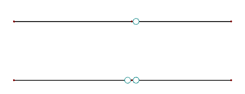
Therefore, it is necessary always to assign one less hinge than members with the same degree of freedom (h = m − 1) at a node. Image 02 shows a valid definition (top) and an invalid definition (bottom).

Member Hinge Members: Top Correct, Bottom Incorrect

End Releases Between Surfaces

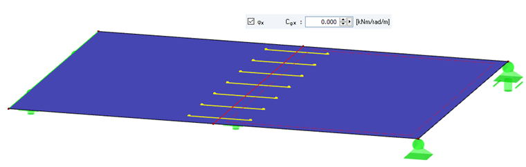
The definition of end releases between surfaces is more complex, but is the same procedure as with members. Here also, two hinges generate a statically underdetermined structure with an identical degree of freedom at a line. Contrary to members, structures including surfaces are not unstable as quickly. This is due in part to the fact that surfaces may warp in their plane and are, therefore, no longer kinematic. Basically, when defining the hinges in Image 03, the line will rotate around its own axis and the structure will, therefore, be kinematic.

Kinematic Line Due to Two Hinges

Joint – Concrete Structures

The simplest case of line hinges is the joint between concrete surfaces mentioned above. It is used to model the assembly gap, which is often necessary in concrete structures.
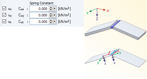
The line hinges in u_x, u_y, and u_z are released for this purpose (Image 04). In this case we recommend releasing the rotation of the line as well. The degree of freedom that is released has to be selected for members and surfaces with hinges.

Structural System Joint

Semi-Rigid Joint – Timber Structures

In timber structures, for example in cross-laminated timber or wood-based panel structures, the separation between surfaces is usually carried out flexibly. It is very easy to consider a linear spring between two surfaces using line hinges. However, the spring in timber structures is actually only available in the tensile direction of the surface. In the contact area between the surfaces, wood-based panels, or cross-laminated timber panels is an almost rigid pressure contact transmission. Thus, modeling such end releases is much more complex, since nonlinear properties have to be considered.

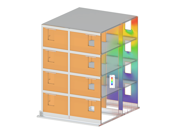
Nonlinear properties have disadvantages in terms of modeling, result evaluation, calculation time, number of unknowns, and so on. In the following text, we explain how it is possible to consider the nonlinearity pressure contact with linear line hinges. Image 05 shows a structure consisting of four surfaces that are connected semi-rigidly. At the support node, the models have free supports in u_x. On the left, a surface is connected semi-rigidly with the fictive springs u_x = 100 kN/m² (longitudinal direction of the line) and u_y = 100 kN/m² (perpendicular to the line). On the right, the direction u_x = 100 kN/m² is connected identically. In u_y, the end release is rigid. At the head, the horizontal load is 15 kN/m.

Comparison Stiffnesses

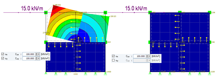
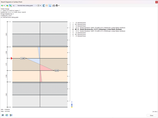
As you can see in Image 05, the deformation of the left model is far too high. In addition, the upper surfaces intersect the lower surfaces. This deformation will not occur like this in practice. However, the deformation of the right model seems plausible. Image 06 shows the shear strain n_xy between the surfaces. The design of the fasteners is carried out for this value. Regardless of the values, you can see that the shear strain of the left model always has a post-critical failure in both directions (positive and negative). This is due to the fact that the results of both surface sides are displayed and both sides consider the end release at the hinge. The shear strain reduces from the center towards the edge at the right model. This results from the overlapping of the stiffnesses inside the connected surfaces.

Shear Strain nxy for Line Hinges

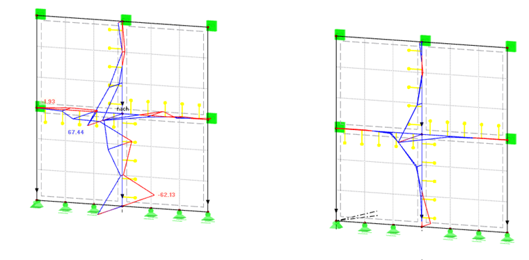
Image 07 shows the force in n_y-direction. The forces displayed at the lines refer in each case to the orientation of the local surface axes.

Forces in ny-Direction

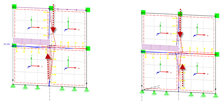
The direction of the force is displayed with dotted red and violet arrows in Image 07. The left model has a disturbed axial force distribution in the vertical axis, which even results in a post-critical failure with the tension component in the lower part. The left model has very high tension forces in the y-direction when looking at the horizontal axis. The axial force increment in the vertical axis starts at zero and increases to the center in the right model. The forces in the horizontal axis are minimal. The force distribution of the right model is thus the most plausible.

Theory for Line Release and Line Hinge

RFEM offers the option to define line releases to consider the nonlinearity of the above-mentioned model, for example in the area of the pressure contact transmission. The theoretical basics are the same for line hinges and line releases. Both are subject to the double node technology. By defining the release, virtually double nodes at the original nodes are generated. These nodes are then connected with each other by means of a spring. As soon as additional nonlinearities (for example, pressure contact) are defined at this spring, a deformation alignment will be performed to check if the condition has been met. The technical term for this method is Penalty Method. Image 08 shows a schematic view.

Penalty Method [1]

You can also carry out alignment based on force. The nonlinearity shown in Image 08 is controlled by the forces in the corresponding direction. Equation 1 shows a schematic view of the equation system for the penalty stiffness k in N/m. Additional derivation and an explanation of the present structure are not included in this article.

Equation 1:

Equation 2 shows the identical equation system with Lagrange multipliers.

Equation 2:

The equation systems only differ in the last part by the factor λ. It is clear now that the calculation with Penalty or Lagrange multipliers leads to identical results, at least in the first step. For more complex structures, it is better to use the Lagrange multipliers. After the start value zero, the iteration scheme is extended by the Langrange multipliers

Line Release

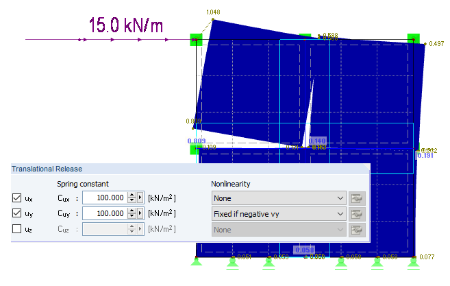
By defining a line release in RFEM, it is possible to fully consider a nonlinearity for the above-mentioned example. As with the rigid model with end release in u_x, a comparable deformation occurs for the identical end release of the nonlinearity pressure contact (Image 09).

Deformation for Line Releases

The internal forces n_xy have an identical distribution of internal forces with regard to the vertical connection, like the structure with only one end release (Image 10). Only the horizontal line changes at the right side of the model, because this surface is completely under pressure.

Shear Distortion for Line Releases

Defining Surface Side

Irrespective of selecting a line release or line hinge for defining the end release, it is important to display the model properly.

Real Model

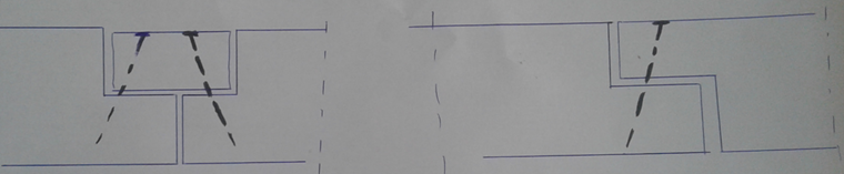
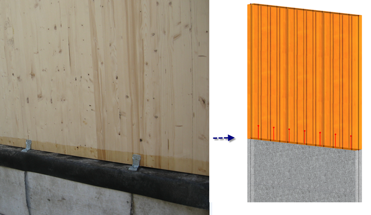
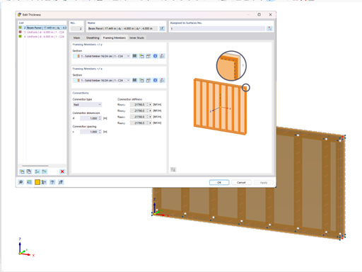
Image 11 shows the nailing with cover panel (left) and notch (right). Image 12 shows the corresponding structural model. When the structure is modeled, it is important to define the end release in u_x, thus in the longitudinal direction of the connection, twice on the left and only once on the right. Due to Hooke's law, the left model has a double end release.

Static System

Summary

Use the option line release or line hinge in RFEM to consider end release between surfaces. Result evaluation and modeling of the system are easier when you calculate with a line hinge. Inaccurate results might be the result. In addition to considering the end release between surfaces, the line release also offers the release of members on surfaces.