62 Wyniki
Wyświetl wyniki:
Sortuj według:
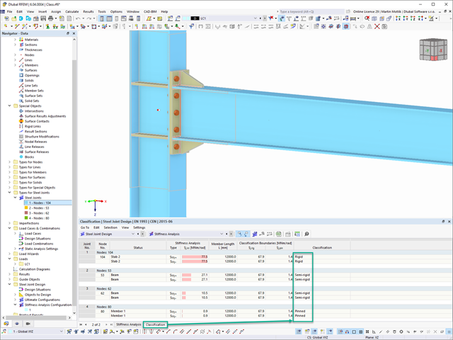
W rozszerzeniu Połączenia stalowe można klasyfikować sztywności połączeń.
Oprócz sztywności początkowej w tabeli wyświetlane są również wartości graniczne dla połączeń przegubowych i sztywnych dla wybranych sił wewnętrznych N, My i/lub Mz. Uzyskana klasyfikacja jest następnie wyświetlana w tabeli jako „przegubowa”, „półsztywna” i „sztywna”.
Przejdź do filmu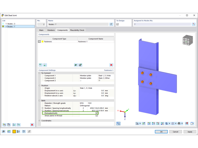
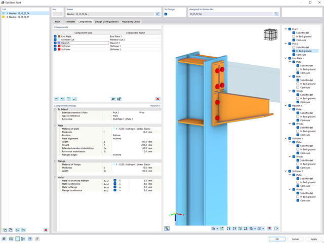
W rozszerzeniu „Połączenia stalowe” można uwzględnić naprężenie wstępne śrub w obliczeniach dla wszystkich komponentów. Sprężenie można łatwo aktywować za pomocą pola wyboru w parametrach śruby i ma ono wpływ zarówno na analizę naprężeniowo-odkształceniową, jak i na analizę sztywności.
Śruby sprężone to specjalne śruby stosowane w konstrukcjach stalowych w celu wygenerowania dużej siły zaciskowej między połączonymi elementami konstrukcyjnymi. Ta siła docisku powoduje tarcie między elementami konstrukcyjnymi, co umożliwia przenoszenie sił.
Funkcjonalność
Śruby sprężane są dokręcane z określonym momentem, co powoduje ich rozciąganie i powstawanie siły rozciągającej. Ta siła rozciągająca jest przenoszona na połączone elementy i prowadzi do powstania dużej siły mocującej. Siła zaciskowa zapobiega poluzowaniu połączenia i zapewnia niezawodne przenoszenie siły.
Zalety
- Wysoka nośność: Śruby wstępnie rozciągane mogą przenosić duże siły.
- Niskie odkształcenie: Minimalizują odkształcenie połączenia.
- Wytrzymałość zmęczeniowa: Są odporne na zmęczenie.
- Łatwość montażu: Są one stosunkowo łatwe w montażu i demontażu.
Analiza i wymiarowanie
Obliczenia śrub sprężanych są przeprowadzane w RFEM z wykorzystaniem modelu analitycznego ES wygenerowanego przez rozszerzenie "Połączenia stalowe". Uwzględnia ona siłę zwarcia, tarcie między elementami konstrukcyjnymi, wytrzymałość śrub na ścinanie oraz nośność elementów konstrukcyjnych. Wymiarowanie odbywa się zgodnie z DIN EN 1993-1-8 (Eurokod 3) lub amerykańską normą ANSI/AISC 360-16. Utworzony model analityczny wraz z wynikami można zapisać i wykorzystać jako niezależny model w programie RFEM.
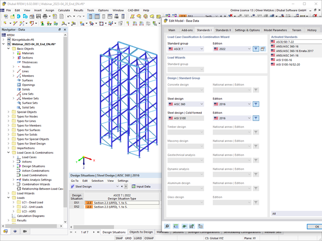
Wymiarowanie prętów stalowych formowanych na zimno zgodnie z AISI S100-16/CSA S136-16 jest dostępne w RFEM 6. Dostęp do obliczeń można uzyskać, wybierając normy „AISC 360” lub „CSA S16” w rozszerzeniu Projektowanie konstrukcji stalowych. Następnie dla obliczeń elementów formowanych na zimno automatycznie wybierane jest „AISI S100” lub „CSA S136”.
Do obliczania sprężystego obciążenia wyboczeniowego pręta program RFEM stosuje metodę DSM. Bezpośrednia metoda wytrzymałości oferuje dwa typy rozwiązań, numeryczne (metoda pasm skończonych) i analityczne (specyfikacja). Krzywą charakterystyczną (sygnaturę) FSM i kształty wyboczenia można wyświetlić w oknie dialogowym Przekroje.
Rozszerzenie Połączenia stalowe umożliwia wymiarowanie połączeń prętów o złożonych przekrojach. Ponadto można przeprowadzać obliczenia połączeń dla prawie wszystkich przekrojów cienkościennych z biblioteki programu RFEM.
Przejdź do filmu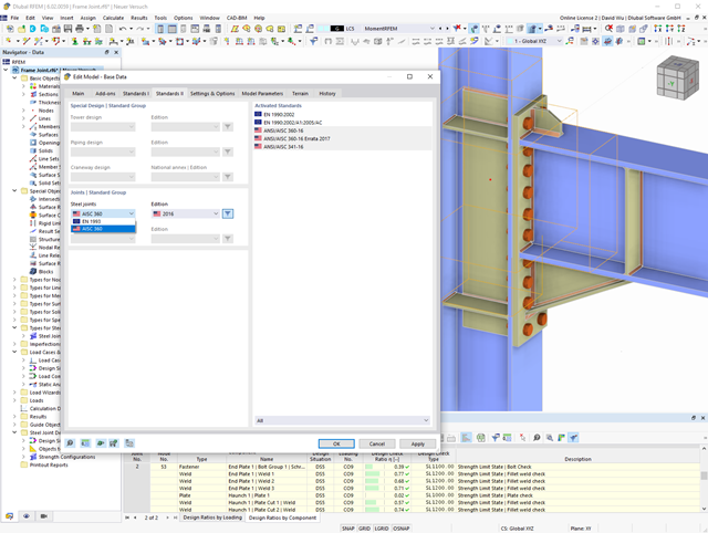
W rozszerzeniu Połączenia stalowe można wymiarować połączenia zgodnie z amerykańską normą ANSI/AISC 360-16. Zintegrowane zostały następujące metody obliczeń:
- Obliczenia współczynnika obciążenia i odporności (LRFD)
- Projektowanie dopuszczalnych naprężeń (ASD)
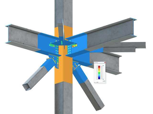
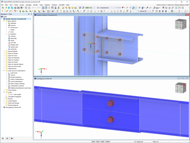
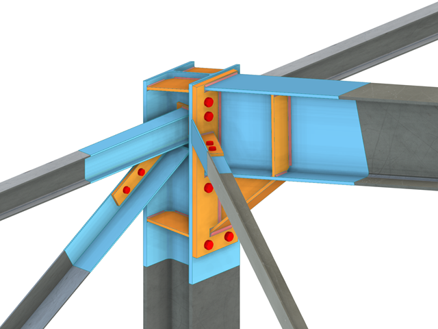
Złożone połączenie belek poziomych ze słupem oraz połączenie stężeń ukośnych
Model połączenia został zamodelowany przy użyciu około 50 komponentów. Model został stworzony na podstawie rzeczywistego przykładu wykorzystania w konstrukcji.
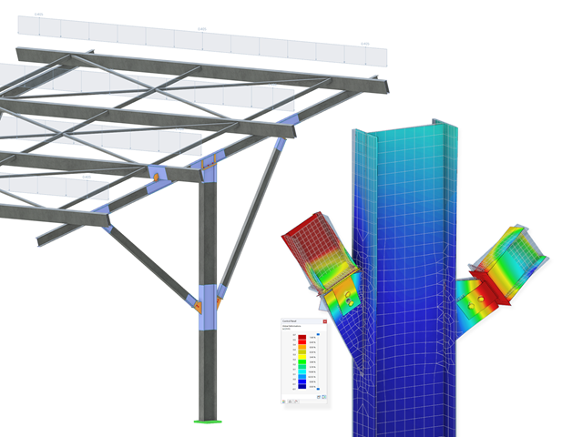
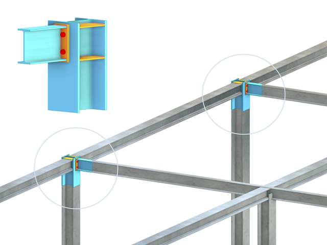
Stalowe połączenia śrubowe z blachami węzłowymi na konstrukcji zadaszenia.
Pobierz model do analizy statyczno-wytrzymałościowej i otwórz go w programie RFEM 6, korzystając z rozszerzenia Połączenia stalowe.
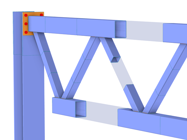
W przypadku przekrojów prostokątnych zwykle można uzyskać bezpośrednie połączenie za pomocą spoin. W ten sam sposób można je jednak połączyć z innymi przekrojami. Ponadto inne elementy, takie jak blachy czołowe, pomagają w łączeniu przekrojów prostokątnych z innymi elementami konstrukcyjnymi.
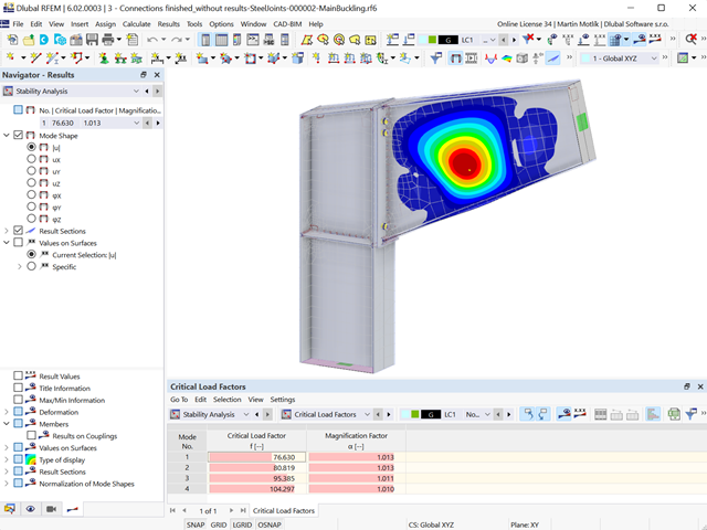
Wymiarowanie połączenia ramy o prętach zbieżnych i usztywnionych. Dla połączenia przeprowadzono analizę naprężeń i stateczności przy wyboczeniu. Aby wyświetlić wyniki dla wyboczenia, połączenie zostało przekształcone w osobny model.
- Proponowane połączenie można zastosować do wszystkich wybranych węzłów w konstrukcji
- Położenie połączenia można zdefiniować w zakładce 'Główne' okna dialogowego rozszerzenia
- Obliczenia są przeprowadzane dla wszystkich połączeń w konstrukcji, a po zakończeniu obliczeń wyniki mogą być wyświetlane we wszystkich połączeniach
- W tabeli wyświetlane są wyniki dla poszczególnych połączeń, każde połączenie jest obliczane i może być zapisane osobno
- Elementy łączące są obliczane zgodnie z AISC 360-16 i Eurokodem EN 1993-1-8.
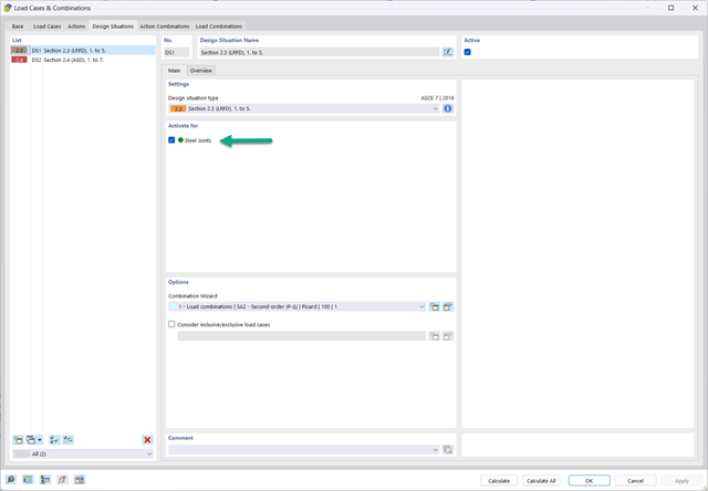
- Po aktywacji rozszerzenia sytuacje obliczeniowe dla połączeń stalowych należy aktywować w oknie dialogowym „Przypadki obciążeń i kombinacje”.
- Do obliczenia stateczności (wyboczenia) połączenia wymagane jest rozszerzenie 'Stateczność konstrukcji'.
- Obliczenia można uruchomić za pomocą tabeli lub ikony w górnym pasku.
- Model połączeń stalowych i wyniki można zapisać jako osobny plik modelu
- Uzyskane naprężenia i wyniki analizy stateczności (wyboczenia połączenia) można wyświetlić w osobnym modelu
- W zapisanym modelu można uruchomić animację deformacji połączenia
- Elementy połączenia są podczas zapisywania przekształcane w powierzchnie i pręty
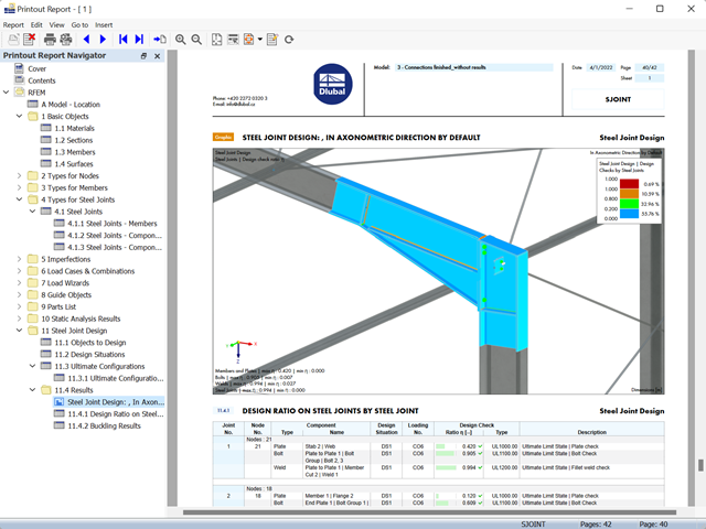
- Wyniki wymiarowania połączeń można wprowadzić do protokołu wydruku
- Podczas tworzenia nowego protokołu wydruku należy wybrać elementy dodane z rozszerzenia Połączenia stalowe
- Za pomocą narzędzia 'Drukowanie grafik do protokołu' można wstawić do protokołu grafikę z wynikami połączenia, w tym z panelem sterowania.
- Protokół wydruku zawiera specyfikacje elementów połączenia, parametry obliczeniowe, wyniki i grafiki
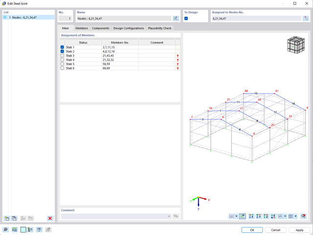
- W przypadku nowego modelu połączenia należy wybrać węzeł w modelu RFEM
- Po wybraniu węzła pręty połączone z węzłem są automatycznie rozpoznawane i przydzielane
- W oknie służącym do przydzielania prętów należy wybrać pręty, które zostaną przydzielone do połączenia
- Zaznaczone przez nas pręty są wyświetlane w oknie podglądu po prawej stronie
- Połączenia mogą być modelowane dla wielu węzłów w konstrukcji.
- Jako ustawienia prętów należy wybrać te, które mają być podparte
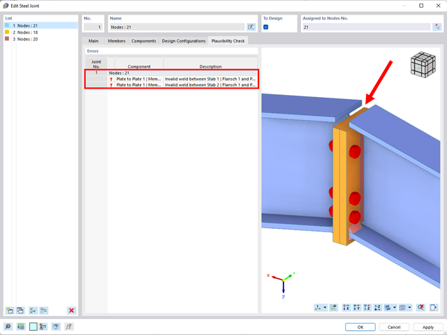
- Równolegle do wprowadzania danych program przeprowadza kontrolę poprawności, aby szybko wykryć brakujące dane wejściowe lub kolizje.
- W przypadku błędu pojawia się komunikat opisujący problem.
W przypadku elementów połączenia można sprawdzić, czy utrata stateczności jest istotna. Wymaga to rozszerzenia Stateczność konstrukcji.
Współczynnik obciążenia krytycznego obliczany jest dla wszystkich analizowanych kombinacji obciążeń oraz wybranej liczby postaci własnych dla modelu połączenia. Porównaj najmniejszy współczynnik obciążenia krytycznego z wartością graniczną 15 z normy EN 1993-1-1, rozdz. 5. Ponadto użytkownik może samodzielnie dostosować wartość graniczną. Wynikiem analizy stateczności jest wyświetlenie w programie graficznej postaci odpowiednich postaci drgań.
Na potrzeby analizy stateczności dostosowany model powierzchniowy jest wykorzystywany w programie RFEM do rozpoznania lokalnych kształtów wyboczeniowych. Można również zapisać model analizy stateczności wraz z wynikami i wykorzystać jako osobny plik modelu.
_(1).png?mw=640&hash=415f7bbaf70e41679bb0106e1cf91eaa8c493ec9)
- Automatyczne generowanie modeli do analizy ES: rozszerzenie automatycznie tworzy w tle model elementów skończonych (ES) połączenia stalowego.
- Uwzględnienie wszystkich sił wewnętrznych: Obliczenia obejmują wszystkie siły wewnętrzne (N , Vy, Vz ,My, Mz, MT ) i nie są ograniczone do obciążeń płaskich.
- Automatyczne przenoszenie obciążeń: Wszystkie kombinacje obciążeń są automatycznie przenoszone do modelu analitycznego ES połączenia. Obciążenia są przenoszone bezpośrednio z programu RFEM, dzięki czemu ręczne wprowadzanie danych nie jest konieczne.
- Wydajne modelowanie: Rozszerzenie pozwala zaoszczędzić czas podczas modelowania złożonych sytuacji związanych z połączeniami. Utworzony model analityczny ES można również zapisać i wykorzystać do własnych szczegółowych analiz.
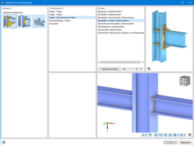
- Rozszerzalna biblioteka: Dostępna jest obszerna, rozszerzalna biblioteka zawierająca wstępnie zdefiniowane szablony połączeń stalowych.
- Szerokie zastosowanie: Rozszerzenie jest odpowiednie do tworzenia połączeń każdego typu i kształtu, jest kompatybilne z prawie wszystkimi przekrojami walcowanymi, spawanymi, złożonymi i cienkościennymi.
- Wybór węzłów w modelu RFEM, automatyczne rozpoznawanie i przydzielanie prętów połączonych z wybranym węzłem
- Dostępnych jest wiele wstępnie zdefiniowanych elementów ułatwiających wprowadzanie typowych komponentów połączeń (np. blachy czołowe, żebra usztywniające)
- Uniwersalne komponenty bazowe (płyty, spoiny, płaszczyzny pomocnicze) do odwzorowania złożonych geometrii połączeń
- Użytkownik nie musi ręcznie edytować modelu MES połączenia, podstawowe ustawienia obliczeń można zmienić w oknie konfiguracji połączenia
- Automatyczne dostosowywanie geometrii połączenia, nawet w przypadku późniejszej edycji prętów, z uwagi na parametryczną definicję położenia komponentów względem siebie
- Równolegle do wprowadzania danych program przeprowadza kontrolę poprawności, aby szybko wykryć brakujące dane wejściowe lub kolizje elementów.
- Wizualizacja geometrii połączenia, która jest aktualizowana równolegle z wprowadzaniem danych
Program wspiera Cię: Moduł określa siły w śrubach na podstawie modelu analitycznego ES i analizuje je automatycznie. Rozszerzenie przeprowadza obliczenia nośności śrub dla przypadków uszkodzeń, takich jak rozciąganie, ścinanie, docisk otworu i przebicie, zgodnie z normą i wyświetla w przejrzysty sposób wszystkie wymagane współczynniki.
Chcesz przeprowadzić wymiarowanie spoin? Spoiny są modelowane jako sprężysto-plastyczne elementy powierzchniowe, a ich naprężenia są odczytywane z modelu analitycznego ES. Kryterium plastyczności ma reprezentować zniszczenie zgodnie z AISC J2-4, J2-5 (wytrzymałość spoin) i J2-2 (wytrzymałość metalu podstawowego). Obliczenia można przeprowadzić z zastosowaniem częściowych współczynników bezpieczeństwa określonych w załączniku krajowym do normy EN 1993-1-8.
Płyty w połączeniu są wymiarowane w sposób plastyczny poprzez porównanie istniejącego odkształcenia plastycznego z dopuszczalnym odkształceniem plastycznym. Domyślne ustawienie wynosi 5% zgodnie z EN 1993-1-5, Załącznik C, ale można to zmienić według specyfikacji użytkownika, a także 5% dla AISC 360.
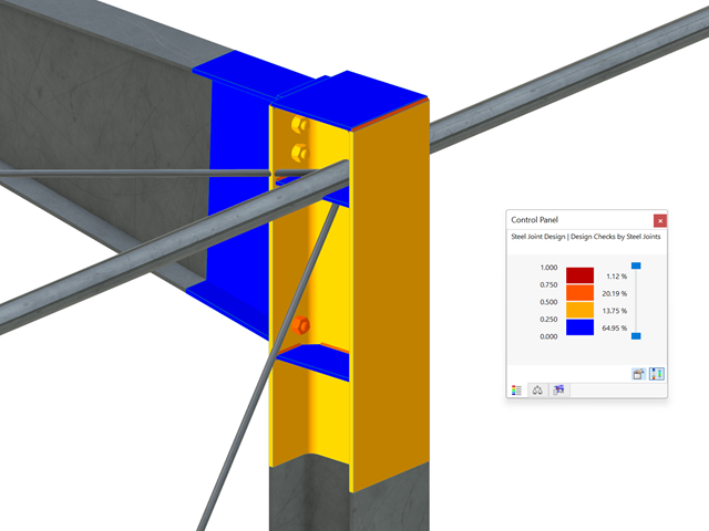
Wszystkie istotne wyniki można wyświetlić w modelu ES. W takim przypadku można filtrować wyniki osobno według odpowiednich komponentów.
Ponadto program RFEM zapewnia wszystkie kontrole obliczeń w formie tabelarycznej wraz z wyświetlaniem zastosowanych wzorów. W razie potrzeby tabele wyników można przenieść do protokołu wydruku programu RFEM.
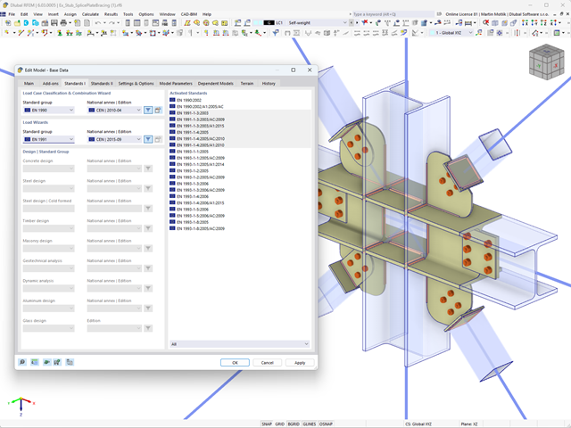
Parametry załączników krajowych (NA) do Eurokodu 3 z następujących krajów są zintegrowane:
-
 DIN EN 1993-1-1/NA:2016-04 (Niemcy)
 -
 ÖNORM EN 1993-1-1/NA:2015-12 (Austria)
 -
 SN EN 1993-1-1/NA:2016-07 (Szwajcaria)
 -
 BDS EN 1993-1-1/NA:2015-10 (Bułgaria)
 -
 BS EN 1993-1-1/NA:2016-07 (Wielka Brytania)
 -
 CEN EN 1993-1-1/2015-06 (Unia Europejska)
 -
 CYS EN 1993-1-1/NA:2015-07 (Cypr)
 -
 CSN EN 1993-1-1/NA:2016-06 (Republika Czeska)
 -
 DS EN 1993-1-1/NA:2015-07 (Dania)
 -
 ELOT EN 1993-1-1/NA:2017-01 (Grecja)
 -
 EVS EN 1993-1-1/NA:2015-08 (Estonia)
 -
 HRN EN 1993-1-1/NA:2016-03 (Chorwacja)
 -
 I S. EN 1993-1-1/NA:2016-03 (Irlandia)
 -
 ILNAS EN 1993-1-1/NA:2015-06 (Luksemburg)
 -
 IST EN 1993-1-1/NA:2015-11 (Islandia)
 -
 LST EN 1993-1-1/NA:2017-01 (Litwa)
 -
 LVS EN 1993-1-1/NA:2015-10 (Łotwa)
 -
 MS EN 1993-1-1/NA:2010-01 (Malezja)
 -
 MSZ EN 1993-1-1/NA:2015-11 (Węgry)
 -
 NBN EN 1993-1-1/NA:2015-07 (Belgia)
 -
 NEN EN 1993-1-1/NA:2016-12 (Holandia)
 -
 NF EN 1993-1-1/NA:2016-02 (Francja)
 -
 NP EN 1993-1-1/NA:2009-03 (Portugalia)
 -
 NS EN 1993-1-1/NA:2015-09 (Norwegia)
 -
 PN EN 1993-1-1/NA:2015-08 (Polska)
 -
 SFS EN 1993-1-1/NA:2015-08 (Finlandia)
 -
 SIST EN 1993-1-1/NA:2016-09 (Słowenia)
 -
 SR EN 1993-1-1/NA:2016-04 (Rumunia)
 -
 SS EN 1993-1-1/NA:2019-05 (Singapur)
 -
 SS EN 1993-1-1/NA:2015-06 (Szwecja)
 -
 STN EN 1993-1-1/NA:2015-10 (Słowacja)
 -
 TKP EN 1993-1-1/NA:2015-04 (Białoruś)
 -
 UNE EN 1993-1-1/NA:2016-02 (Hiszpania)
 -
 UNI EN 1993-1-1/NA:2015-08 (Włochy)
- 002089
- Ogólne informacje
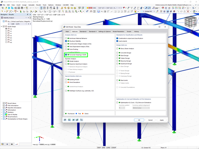
- Skręcanie skrępowane (7 stopni swobody) RFEM 6
- Skręcanie skrępowane (7 stopni swobody) RSTAB 9
- Uwzględnienie 7 lokalnych kierunków deformacji (ux , uy, uz, φx, φy, φz, ω ) lub 8 sił wewnętrznych (N , Vu, Vv, Mt, pri, Mt, s, Mu, Mv, Mω ) przy obliczaniu elementów prętowych
- Możliwość stosowania w połączeniu z analizą statyczno-wytrzymałościową według teorii II rzędu, i analiza dużych deformacji (można również uwzględnić imperfekcje)
- W połączeniu z rozszerzeniem Analiza stateczności umożliwia definiowanie współczynników obciążenia krytycznego i kształtów drgań dla problemów stateczności, takich jak wyboczenie skrętne i zwichrzenie
- Uwzględnianie blach czołowych i usztywnień poprzecznych jako sprężystości skrępowanej podczas obliczania przekrojów dwuteowych z automatycznym określaniem i wyświetlaniem graficznym sztywności sprężystości deplanacyjnej
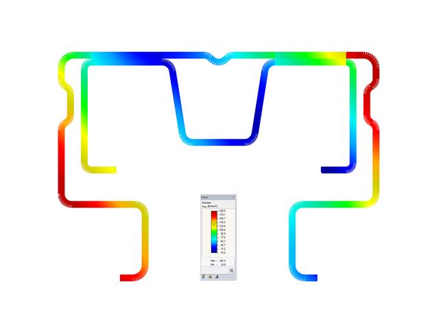
- Graficzne przedstawienie deplanacji przekroju prętów w stanie odkształcenia
- Pełna integracja z RFEM i RSTAB

- 002090
- Ogólne informacje
- Skręcanie skrępowane (7 stopni swobody) RFEM 6
- Skręcanie skrępowane (7 stopni swobody) RSTAB 9
Obliczenia skręcania skrępowanego można przeprowadzić dla całego układu. Uwzględniasz zatem dodatkową wartość 7 stopnia swobody w obliczeniach pręta. Sztywności połączonych elementów konstrukcyjnych są uwzględniane automatycznie. Oznacza to, że nie ma potrzeby' definiowania równoważnych sztywności sprężystych ani warunków podparcia dla układu odłączanego.
Następnie można wykorzystać siły wewnętrzne z obliczeń ze skręcaniem skrępowanym w rozszerzeniu do obliczeń. W zależności od materiału i wybranej normy należy uwzględnić bimoment wyboczeniowy i drugorzędny moment skręcający. Typowym zastosowaniem jest analiza stateczności według teorii drugiego rzędu z wykorzystaniem imperfekcji w konstrukcjach stalowych.
Czy wiecie, że...? Zastosowanie nie ogranicza się do przekrojów stalowych cienkościennych. Pozwala to na przykład na przeprowadzenie obliczeń idealnego momentu krytycznego dla belek o przekrojach z drewna litego.
- 002401
- Ogólne informacje
- Skręcanie skrępowane (7 stopni swobody) RFEM 6
- Skręcanie skrępowane (7 stopni swobody) RSTAB 9
- Funkcję skręcania skrępowanego można aktywować lub dezaktywować w zakładce Rozszerzenia w Danych podstawowych modelu.
- Po aktywowaniu rozszerzenia interfejs użytkownika w programie RFEM zostaje rozszerzony o nowe wpisy w nawigatorze, tabelach i oknach dialogowych.
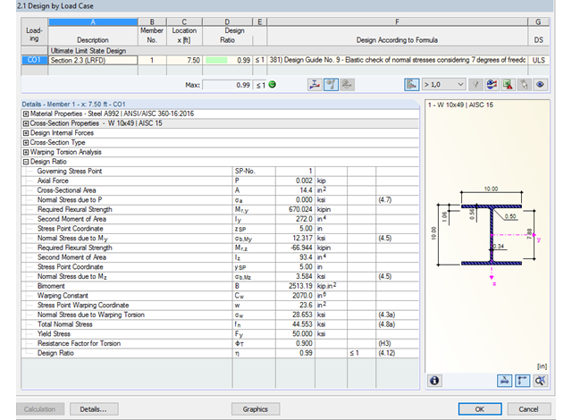
Dzięki zintegrowanemu rozszerzeniu modułu RF-/STEEL Warping Torsion, możliwe jest przeprowadzenie obliczeń zgodnie z Design Guide 9 w RF-/STEEL AISC.
Obliczenia są przeprowadzane z 7 stopniami swobody zgodnie z teorią skręcania skrępowanego i umożliwiają realistyczne obliczenia stateczności z uwzględnieniem skręcania.
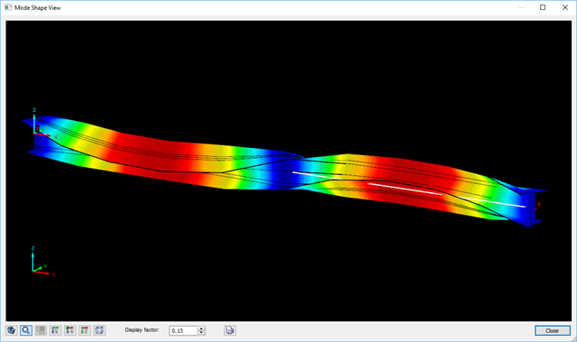
Definiowanie krytycznego momentu wyboczeniowego odbywa się w module RF-/STEEL AISC za pomocą solwera wartości własnych, który umożliwia dokładne określenie krytycznego obciążenia wyboczeniowego.
Solwer wartości własnych pokazuje okno z grafiką wartości własnych, które umożliwia sprawdzenie warunków brzegowych.
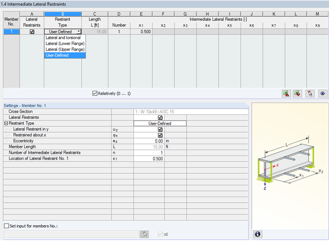
W programie STEEL AISC możliwe jest uwzględnienie pośrednich podpór bocznych w dowolnym miejscu. Na przykład, możliwa jest stabilizacja tylko górnej półki.
Ponadto można przypisać boczne podpory pośrednie zdefiniowane przez użytkownika; na przykład pojedyncze sprężyny obrotowe i sprężyny translacyjne w dowolnym miejscu przekroju.
- Modelowanie przekroju za pomocą elementów, profili, łuków i elementów punktowych
- Biblioteka właściwości materiałów, granic plastyczności i naprężeń granicznych, którą użytkownik może rozbudowywać
- Właściwości przekrojów otwartych, zamkniętych i niepołączonych
- Efektywne właściwości przekrojów wykonanych z różnych materiałów
- Określanie naprężeń w spoinach pachwinowych
- Analiza naprężeń wraz z obliczaniem skręcania swobodnego i skrępowanego
- Sprawdzanie stosunków (c/t)
- Przekroje efektywne według
- EN 1993-1-5 (w tym płyty usztywnione zgodnie z rozdziałem 4.5)
-
EN 1993-1-3
-
EN 1999-1-1
-
DIN 18800-2
- Klasyfikacja według
-
EN 1993-1-1
-
EN 1999-1-1
-
- Interfejs z MS Excel służący do importu i eksportu tabel
- Raport
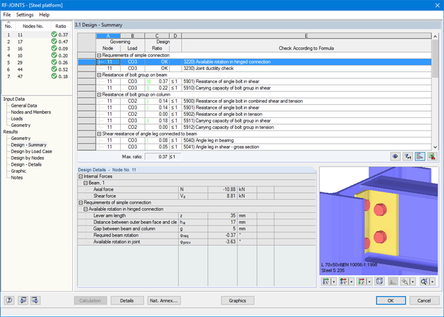
W oknach wyników wyszczególnione są wszystkie wyniki obliczeń. Ponadto tworzone są grafiki 3D, w których poszczególne elementy oraz linie wymiarowe można wyświetlać lub ukrywać. W podsumowaniu można sprawdzić, czy potwierdzono poprawność obliczeń: Stopień wykorzystania jest dodatkowo wizualizowany za pomocą zielonego paska danych, który zmienia kolor na czerwony, gdy obliczenia nie są spełnione. Ponadto wyświetlany jest numer węzła i decydujące PO/KO/KW.
Podczas wyboru obliczeń wyświetlane są szczegółowe wyniki pośrednie wraz z oddziaływaniami i dodatkowymi siłami wewnętrznymi wynikającymi z geometrii połączenia. Istnieje możliwość wyświetlenia wyników według przypadków obciążeń i węzłów. Połączenia są przedstawione w realistycznym renderingu 3D, który można skalować. Oprócz głównych widoków, połączenie można zobaczyć z każdej strony.
Grafiki z wymiarami i opisami można dodać do wydruku programu RFEM/RSTAB lub eksportować jako DXF. Protokół wydruku zawiera wszystkie dane wejściowe i wyniki, przygotowane dla inżynierów testujących. Wszystkie tabele można wyeksportować do programu MS Excel lub do pliku CSV. Wszystkie dane wymagane do eksportu definiuje się w specjalnym menu dla transferu.
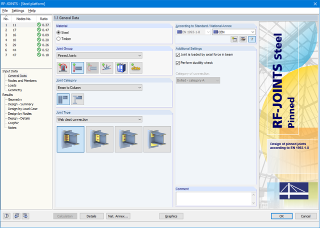
Po otwarciu modułu należy wybrać grupę połączeń (Połączenia przegubowe), następnie kategorię oraz typ połączenia (środnik nakładkowy, blacha zakładkowa, blacha czołowa, blacha czołowa z podkładką). Następnie można wybrać węzły do obliczeń w modelu RFEM/RSTAB. RF-/JOINTS Steel - Pinned automatycznie rozpoznaje pręty połączenia i określa na podstawie ich położenia, czy są to słupy czy belki.
W razie potrzeby można wyłączyć określone pręty z obliczeń. Konstrukcyjnie podobne połączenia można projektować jednocześnie dla kilku węzłów. Obciążenia wymagają wyboru miarodajnych przypadków obciążeń, kombinacji obciążeń lub kombinacji wyników. Alternatywnie można ręcznie wprowadzić przekrój i obciążenie. W ostatnim oknie wprowadzania danych połączenie jest konfigurowane krok po kroku.