21 Wyniki
Wyświetl wyniki:
Sortuj według:
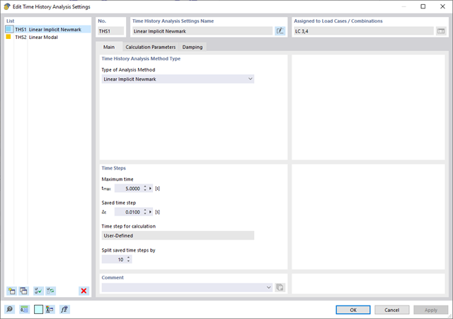
Analiza historii czasowej rozwiązywana jest za pomocą analizy modalnej lub metodą Newmarka. Analiza historii czasowej w tym rozszerzeniu jest ograniczona do układów liniowych. Chociaż modalna analiza jest szybkim algorytmem, pewna liczba wartości własnych musi być stosowana w celu zapewnienia wymaganej dokładności wyników.
Metoda Newmarka jest bardzo precyzyjną metodą, niezależną od zastosowanej liczby wartości własnych, ale w obliczeniach wymaga odpowiednich niewielkich kroków czasowych.

- Outsourcing obliczeń do serwerów obliczeniowych w chmurze
- Możliwość wyboru spośród różnych wydajnych serwerów obliczeniowych
- Przejrzyste wyświetlanie wszystkich zadań obliczeniowych w Extranecie
- Pliki z obliczeniami będą dostępne do pobrania przez 2 miesiące
- Wirtualnie nieograniczona moc obliczeniowa w chmurze
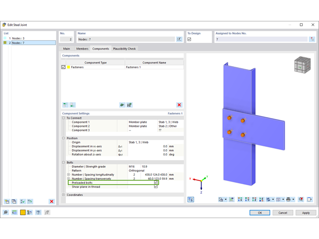
W rozszerzeniu „Połączenia stalowe” można uwzględnić naprężenie wstępne śrub w obliczeniach dla wszystkich komponentów. Sprężenie można łatwo aktywować za pomocą pola wyboru w parametrach śruby i ma ono wpływ zarówno na analizę naprężeniowo-odkształceniową, jak i na analizę sztywności.
Śruby sprężone to specjalne śruby stosowane w konstrukcjach stalowych w celu wygenerowania dużej siły zaciskowej między połączonymi elementami konstrukcyjnymi. Ta siła docisku powoduje tarcie między elementami konstrukcyjnymi, co umożliwia przenoszenie sił.
Funkcjonalność
Śruby sprężane są dokręcane z określonym momentem, co powoduje ich rozciąganie i powstawanie siły rozciągającej. Ta siła rozciągająca jest przenoszona na połączone elementy i prowadzi do powstania dużej siły mocującej. Siła zaciskowa zapobiega poluzowaniu połączenia i zapewnia niezawodne przenoszenie siły.
Zalety
- Wysoka nośność: Śruby wstępnie rozciągane mogą przenosić duże siły.
- Niskie odkształcenie: Minimalizują odkształcenie połączenia.
- Wytrzymałość zmęczeniowa: Są odporne na zmęczenie.
- Łatwość montażu: Są one stosunkowo łatwe w montażu i demontażu.
Analiza i wymiarowanie
Obliczenia śrub sprężanych są przeprowadzane w RFEM z wykorzystaniem modelu analitycznego ES wygenerowanego przez rozszerzenie "Połączenia stalowe". Uwzględnia ona siłę zwarcia, tarcie między elementami konstrukcyjnymi, wytrzymałość śrub na ścinanie oraz nośność elementów konstrukcyjnych. Wymiarowanie odbywa się zgodnie z DIN EN 1993-1-8 (Eurokod 3) lub amerykańską normą ANSI/AISC 360-16. Utworzony model analityczny wraz z wynikami można zapisać i wykorzystać jako niezależny model w programie RFEM.
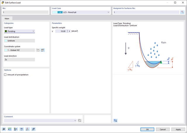
Wprowadzenie typu obciążenia Woda stojąca umożliwia symulację oddziaływań deszczu na powierzchnie wielokrotnie zakrzywione, z uwzględnieniem przemieszczeń według analizy dużych odkształceń.
Ten numeryczny proces analizy deszczowej analizuje przypisaną geometrię powierzchni i określa, które składowe wody deszczowej spływają, a które gromadzą się w postaci kałuży (kieszeni wodnych) na powierzchni. Rozmiar kałuży powoduje wówczas odpowiednie obciążenie pionowe do analizy statyczno-wytrzymałościowej.
Funkcja ta jest przeznaczona do analizy w przybliżeniu poziomych geometrii dachów membranowych pod obciążeniem deszczem.
Przejdź do filmu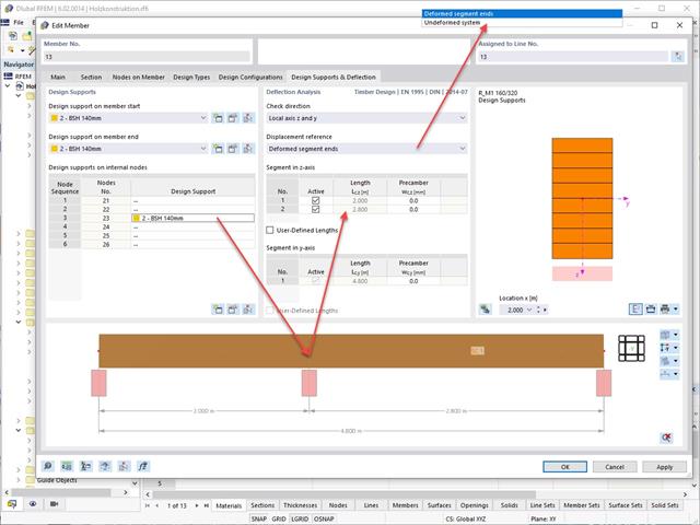
W zakładce 'Podpory obliczeniowe i ugięcia' w pozycji 'Edytować pręt', pręty można podzielić na segmenty za pomocą zoptymalizowanych okien wprowadzania danych. W zależności od warunków podparcia, wartości graniczne odkształceń dla belek wspornikowych lub belek jednoprzęsłowych są dostosowywane automatycznie.
Po zdefiniowaniu podpory obliczeniowej w odpowiednim kierunku na początku pręta, końcu pręta i w węzłach pośrednich, program automatycznie rozpoznaje segmenty i długości segmentów, do których odnosi się dopuszczalne odkształcenie. Na podstawie zdefiniowanych podpór obliczeniowych moduł wykrywa również automatycznie, czy jest to belka czy wspornik. Ręczne przydzielanie, podobnie jak w poprzednich wersjach (RFEM 5), nie jest już konieczne.
Opcja 'Długości zdefiniowane przez użytkownika' umożliwia modyfikowanie długości odniesienia w tabeli. Domyślnie stosowana jest zawsze odpowiednia długość segmentu. Jeżeli długość odniesienia różni się od długości segmentu (na przykład w przypadku prętów zakrzywionych), można ją dostosować.
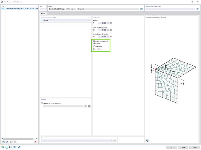
Mamy dla Ciebie'coś nowego! W celu zdefiniowania nieparzystego zagęszczenia siatki, dodano opcje rozmieszczania ES:
- Radialny
- Rozmieść stopniowo
- Sposób mieszany
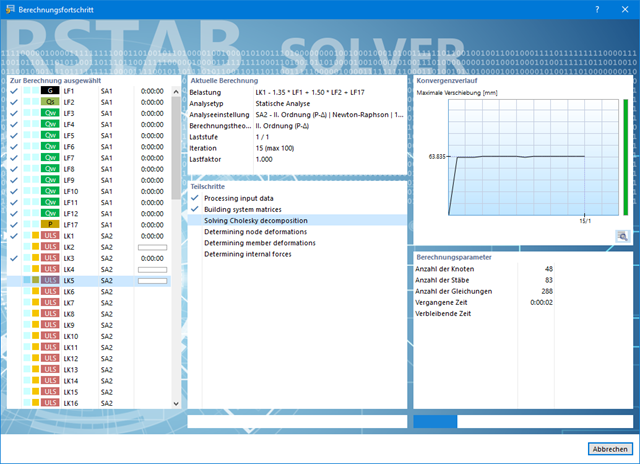
Również w tym przypadku program RSTAB z pewnością Cię przekona. Dzięki wydajnemu jądru obliczeniowemu, zoptymalizowanym połączeniom sieciowym i obsłudze technologii procesorów wielordzeniowych, program do analizy statyczno-wytrzymałościowej firmy Dlubal jest daleko do przodu. Umożliwia to obliczanie bardziej liniowych przypadków obciążeń i kombinacji obciążeń przy użyciu kilku procesorów równolegle, bez konieczności używania dodatkowej pamięci. Macierz sztywności tworzona jest tylko raz. Dzięki temu możliwe jest obliczanie nawet dużych układów za pomocą szybkiego i bezpośredniego solwera.
Musisz obliczyć kilka kombinacji obciążeń w swoich modelach? Program uruchamia równolegle kilka solwerów (po jednym na rdzeń). Następnie każdy solwer oblicza kombinację obciążeń. Prowadzi to do lepszego wykorzystania dostępnych rdzeni.
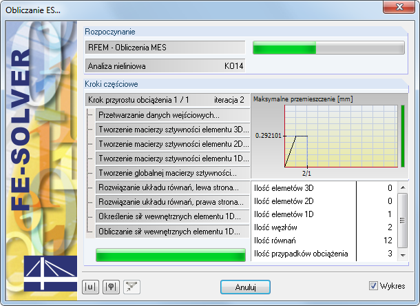
Podczas obliczeń można dokładnie śledzić rozwój odkształcenia na wykresie, a tym samym dokładnie ocenić zachowanie zbieżności.
Przekonaj się do jądra obliczeń, zoptymalizowanej sieci i nieograniczonej obsłudze systemów wieloprocesorowych. Możliwe są równoległe obliczenia liniowych przypadków obciążeń i kombinacji obciążeń przez kilka procesorów jednocześnie bez dodatkowych wymagań dotyczących pamięci RAM. Macierz sztywności tworzona jest tylko raz. Dzięki temu nawet duże układy konstrukcyjne mogą być obliczane za pomocą szybkiego solwera bezpośredniego.
Jeżeli konieczne jest obliczenie wielu kombinacji obciążeń dla modeli, program uruchamia równolegle kilka solwerów (po jednym na każdy rdzeń). Wówczas każdy solwer oblicza kombinację obciążeń, dzięki czemu można lepiej wykorzystać rdzenie.
Podczas obliczeń można dokładnie śledzić rozwój odkształcenia na wykresie, a tym samym dokładnie ocenić zachowanie zbieżności.
.png?mw=640&hash=9aa98962d5e0d0ed2803b35fcb6a2f87288b0946)
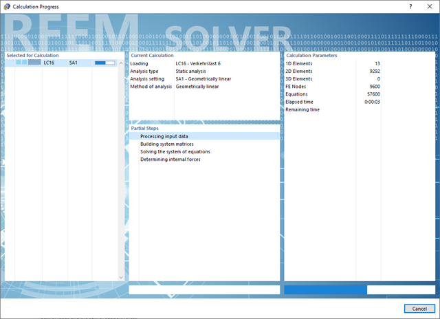
Liczba stopni swobody w węźle nie jest już globalnym parametrem obliczeniowym w programie RFEM (6 stopni swobody dla każdego węzła siatki w modelach 3D, 7 stopni swobody dla analizy skręcania skrępowanego). Dlatego każdy węzeł jest zwykle rozpatrywany z inną liczbą stopni swobody, co prowadzi do zmiennej liczby równań w obliczeniach.
Zmiana ta przyspiesza obliczenia, szczególnie dla modeli, które mogą być znacznie uproszczone, takich jak konstrukcje kratownicowe i membranowe.
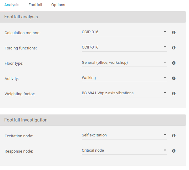
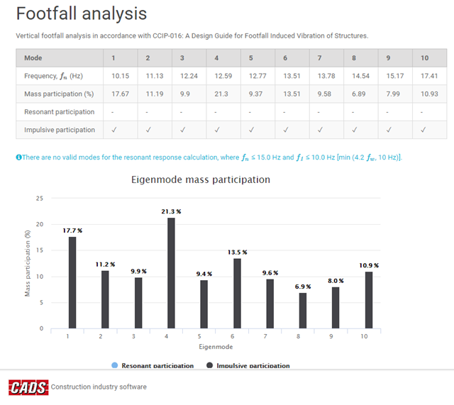
- Analiza Footfall łączy się z programem RFEM, wykorzystując geometrię modelu, dzięki czemu użytkownik nie musi tworzyć drugiego modelu specjalnie do analizy Footfall
- Umożliwia użytkownikowi analizę każdego typu konstrukcji, niezależnie od kształtu, materiału lub zastosowania
- Szybkie i dokładne przewidywanie odpowiedzi rezonansowych i impulsowych (przejściowych)
- Zbiorczy pomiar poziomów drgań – analiza VDV
- Intuicyjne dane wyjściowe, które umożliwiają inżynierowi sugerowanie ulepszeń w krytycznych obszarach w ekonomiczny sposób.
- Ocena przekroczenia wartości granicznych zgodnie z BS 6472 i ISO 10137
- Wybór sił wzbudzających: CCIP-016, SCI P354, AISC DG11 do podłóg i schodów
- Krzywe ważenia częstotliwościowego (BS 6841)
- Szybkie sprawdzenie całego modelu lub określonych obszarów
- Analiza dawki drgań (VDV)
- Regulacja minimalnej i maksymalnej częstotliwości chodzenia oraz wagi pieszego
- Dane wejściowe tłumienia wprowadzane przez użytkownika
- Ustawienie liczby kroków dla odpowiedzi rezonansowej poprzez wprowadzenie danych przez użytkownika lub obliczenie przez program
- Wartość graniczna reakcji środowiskowej w oparciu o BS 6472 i ISO 10137
- Ogólne maksymalne współczynniki odpowiedzi i węzły krytyczne
- Analiza rezonansowa (maksymalny współczynnik odpowiedzi, przyspieszenie RMS, węzeł krytyczny, częstotliwość krytyczna)
- Analiza impulsowa (przejściowa) (maksymalny współczynnik odpowiedzi, szczytowe przyspieszenie/prędkość, RMS przyspieszenie/prędkość, węzeł krytyczny, częstotliwość krytyczna)
- Wartości dawki drgań dla analizy rezonansowej i impulsowej
Wykresy
- Współczynnik odpowiedzi a częstotliwość ruchu pieszego
- Udział masy a postacie własne
- Analiza czasowa prędkości
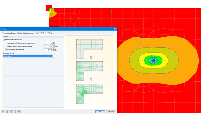
Funkcja ta umożliwia automatyczne zagęszczenie siatki ES na powierzchniach. Zagęszczenie siatki jest stopniowe. Na każdym kroku siatka ES jest tworzona na podstawie porównania błędów wyników w poprzednim kroku obliczeń. Błąd numeryczny jest obliczany na podstawie wyników dla elementów powierzchniowych i jest oparty na sformułowaniu energetycznym Zienkiewicza-Zhu.
Ocena błędu jest przeprowadzana dla liniowej analizy statycznej. Wybieramy przypadek obciążenia (lub kombinację obciążeń), dla którego wygenerowana jest siatka ES. Siatka ES jest następnie wykorzystywana do wszystkich obliczeń.
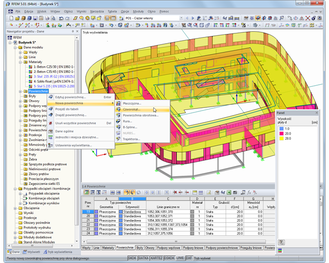
Programy firmy Dlubal są przyjazne dla użytkownika. Zapewnia to krótki czas wdrożenia i łatwą obsługę oprogramowania.
Konstrukcja zostaje utworzona w typowym dla CAD interfejsie użytkownika lub za pomocą tabel. Klikając prawym przyciskiem myszy obiekt graficzny lub obiekt nawigatora, można aktywować menu kontekstowe, które umożliwia łatwe tworzenie lub modyfikowanie obiektów. Wypróbuj i daj się zainspirować intuicyjnemu interfejsowi! Dzięki temu obiekty konstrukcji i obciążeń można utworzyć w bardzo krótkim czasie.
Solver równań zawiera zoptymalizowany generator siatki ES i obsługuje najnowszy procesor wielordzeniowy oraz technologię 64-bitową. Umożliwia równoległe obliczenia liniowych przypadków obciążeń i kombinacji obciążeń przez kilka procesorów jednocześnie bez dodatkowych wymagań dotyczących pamięci RAM: Macierz sztywności tworzona jest tylko raz. Technologia 64-bitowa i rozszerzone opcje pamięci RAM umożliwiają obliczanie złożonych układów konstrukcyjnych przy użyciu szybkiego i bezpośredniego solwera równań.
Podczas obliczeń zmiana odkształceń jest wyświetlany w formie wykresu. Pozwala to na przejrzystą ocenę zachowania zbieżności obliczeń.
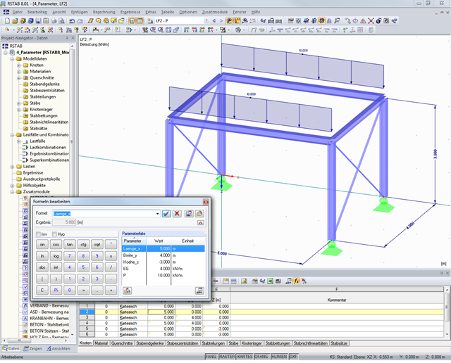
W celu efektywnej edycji powtarzających się układów w programie RFEM można wprowadzać parametryzowaną analizę danych, która może być łączona z metodą parametryzowanych linii pomocniczych. Modele można tworzyć przy użyciu określonych parametrów i dostosowywać do nowej sytuacji poprzez ich modyfikację.
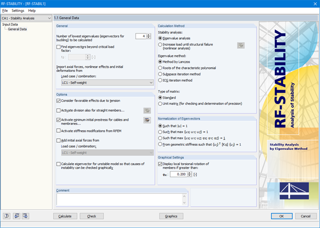
W pierwszej kolejności należy wybrać przypadek lub kombinację obciążeń, którego siły osiowe mają zostać użyte w analizie stateczności. Możliwe jest zdefiniowanie innego przypadku obciążenia, na przykład w celu uwzględnienia wstępnego naprężenia wstępnego.
Następnie można wybrać analizę liniową lub nieliniową, która ma zostać przeprowadzona. W zależności od zastosowania, można skorzystać z bezpośredniej metody obliczeniowej, np. według Lanczosa lub metodą iteracji ICG. Pręty niezintegrowane z powierzchniami są zazwyczaj wyświetlane jako elementy prętowe z dwoma węzłami ES. Nie można określić wyboczenia lokalnego pojedynczych prętów na tych elementach. Dlatego istnieje możliwość automatycznego podziału prętów.
- 002074
- Ogólne informacje
- Analiza stateczności konstrukcji RFEM 6
- Analiza stateczności konstrukcji RSTAB 9
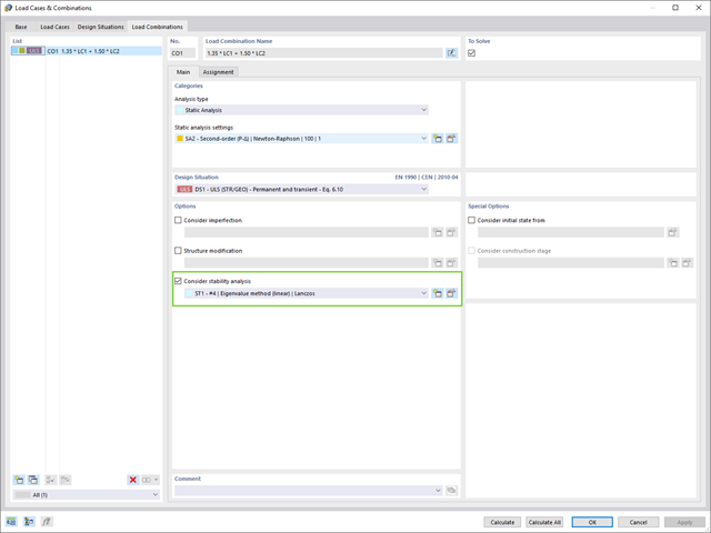
Jeżeli w programie istnieje przypadek obciążenia lub kombinacja obciążeń, obliczenia stateczności są aktywowane. Można zdefiniować inny przypadek obciążenia, na przykład w celu uwzględnienia naprężenia początkowego.
W tym celu należy określić, czy ma zostać przeprowadzona analiza liniowa czy nieliniowa. W zależności od przypadku zastosowania, można wybrać bezpośrednią metodę obliczeniową, taką jak metoda Lanczosa lub metoda iteracji ICG. Pręty niezintegrowane z powierzchniami są zazwyczaj wyświetlane jako elementy prętowe z dwoma węzłami ES. W przypadku zastosowania takich elementów program nie może określić wyboczenia lokalnego pojedynczych prętów. Z tego względu'istnieje możliwość automatycznego dzielenia prętów.
W przypadku globalnego rodzaju obliczeń sztywność obliczona na podstawie wybranego zbioru warstw oraz geometria tafli są przyporządkowane do każdej powierzchni. Obliczenia są przeprowadzana przy użyciu teorii płyt. Zdecydować można także czy uwzględnione będzie ścinanie połączenia warstw.
W przypadku lokalnego rodzaju obliczeń wybrać można pomiędzy obliczeniami 2D lub 3D. Obliczenia dwuwymiarowe oznaczają, że szkło jednowarstwowe lub laminowane jest modelowane jako powierzchnia, której grubość jest obliczana na podstawie wybranej konstrukcji i geometrii szkła (przy użyciu teorii płyt). Podobnie jak w obliczeniach globalnych, ścinanie połączenia warstw może być uwzględnione.
Podczas obliczeń 3D w modelu używane są bryły, które zastępują każdy zbiór warstw. Dzięki temu wyniki są dokładniejsze, ale obliczenia mogą zająć więcej czasu.
Modelowanie szkła zespolonego możliwe jest tylko wtedy, gdy wybrany jest lokalny typ obliczeń. Warstwa gazu jest zawsze modelowana jako element bryłowy, dlatego konieczne jest projektowanie poszczególnych elementów szklanych niezależnie od otaczającej konstrukcji. W obliczeniach i analizie trzeciego rzędu uwzględniane jest równanie stanu gazu doskonałego (cieplne równanie stanu gazów doskonałych).
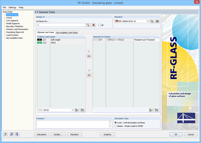
W module dodatkowym należy wybrać powierzchnie, które mają zostać zwymiarowane (na przykład za pomocą funkcji Wybierz). Geometria tafli szkła oraz obciążenia są importowane z modelu RFEM.
Następnie należy zdecydować, czy obliczenia mają być przeprowadzone bez wpływu sąsiedniej konstrukcji (obliczenia lokalne) czy z uwzględnieniem tego wpływu (obliczenia globalne). W przypadku wybrania opcji obliczeń lokalnych każda powierzchnia wybrana do obliczeń zostanie odłączona od modelu i obliczona osobno.
W obliczeniach globalnych uwzględniana jest cała konstrukcja wraz z wprowadzonymi szybami. Wszystkie dane dotyczące składu szkła oraz właściwości szkła poszczególnych warstw należy zdefiniować w oknie wprowadzania danych w module RF-GLASS. Do wyboru są warstwy typu szkło, folia i gaz. Żądany materiał można zaimportować bezpośrednio z biblioteki, która zawiera dużą liczbę materiałów.
Wszystkie parametry poszczególnych warstw, w tym ich grubości, można edytować. Ponadto w RF-GLASS można tworzyć szereg zestawień, co pozwala na wspólne wymiarowanie różnych typów szkła.
W przypadku szkła izolacyjnego w analizie można uwzględnić obciążenia zewnętrzne oraz obciążenia spowodowane zmianami temperatury, ciśnienia atmosferycznego i wysokości. Moduł oblicza te obciążenia automatycznie na podstawie parametrów obciążeń klimatycznych. W przypadku wybrania lokalnego typu obliczeń należy zdefiniować podpory liniowe, podpory węzłowe i pręty graniczne powierzchni w module RF-GLASS. Podpory i pręty są uwzględniane tylko w programie RF-GLASS i nie mają wpływu na model utworzony w programie RFEM.
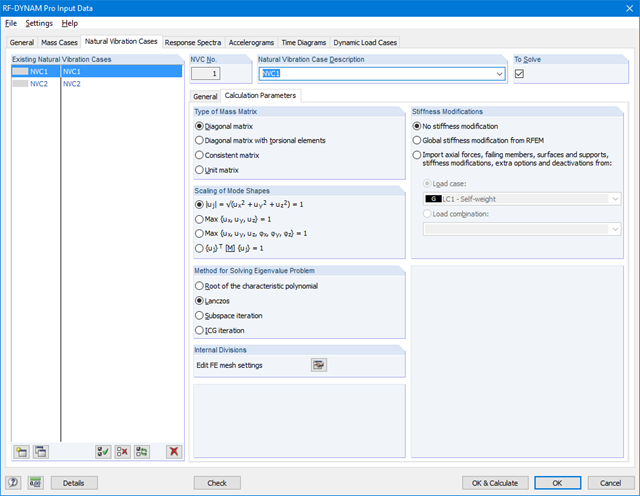
Analiza historii czasowej rozwiązywana jest za pomocą analizy modalnej lub metodą Newmarka. W tym module dodatkowym analiza przebiegu czasowego jest ograniczona do układów liniowych. Chociaż modalna analiza jest szybkim algorytmem, pewna liczba wartości własnych musi być stosowana w celu zapewnienia wymaganej dokładności wyników.
Metoda Newmarka jest bardzo precyzyjną metodą, niezależną od zastosowanej liczby wartości własnych, ale w obliczeniach wymaga odpowiednich niewielkich kroków czasowych. Dla analizy spektrum odpowiedzi równoważne obciążenie statyczne obliczane jest wewnętrznie. Następnie z tej analizy wykonywana jest liniowa analiza statyczna.
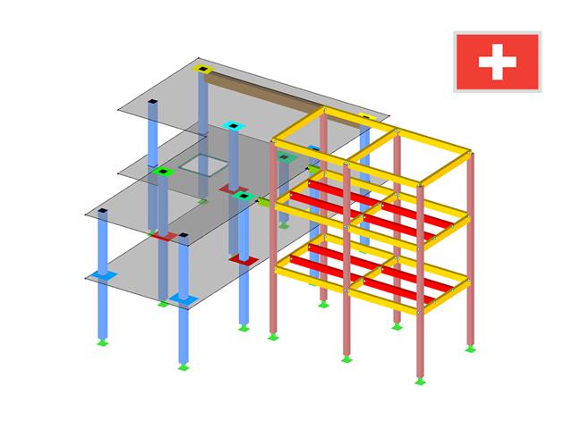
Biblioteka materiałów zapewnia szwajcarskie typy betonu i stali zbrojeniowej. Podczas analizy według SIA 262 możliwe jest również tworzenie własnych materiałów. Program prowadzi obliczenia w stanie granicznym nośności i użytkowalności.
Analiza szerokości rys może być prowadzona poprzez obliczenie ss,adm, poprzez określenie rozstawu prętów zbrojeniowych sL lub poprzez bezpośrednie obliczenie szerokości rys według dokumentacji D0182. Wartość graniczna s s,adm określana jest przez program w zależności od wybranego typu betonu przy użyciu równania 10.13 z dokumentacji D0182, przy górnej granicy określonej przez wartość fsd.