Linear Solver Options
In the Static Analysis Settings, two linear solver options are available in the "Method for Equation System" area – Direct and Iterative.
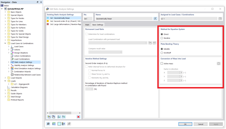
Both options control the method used for solving the equation system; that is, "directly" or "iteratively". To prevent misunderstandings: When solving the equation system directly, an iterative calculation is performed as well if there are nonlinearities, or if data are calculated according to the second-order or large deformation analysis. "Direct" and "Iterative" refer to the data management during the calculation.
In contrast to direct solvers, iterative methods approach problem solutions gradually, as opposed to a single extensive computational step. Consequently, utilizing an iterative method reveals a reduction in solution error estimates with increasing iterations. Convergence for well-conditioned problems typically exhibits a smooth progression, while less well-conditioned problems experience slower convergence. Oscillatory behavior within an iterative solver often signifies improper problem setup, such as insufficient constraints.
One significant advantage of iterative solvers lies in their minimized memory consumption compared to direct solvers when dealing with problems of equivalent size. However, an inherent drawback of iterative solvers is their sensitivity to solver settings, which must be tailored to the specific governing equation's characteristics within distinct physics scenarios. The "Direct" solver option is generally favorable, as long as enough RAM is available.
Recommendations
Which solver method leads to results more quickly depends on the complexity of the model as well as the size of the available main memory (RAM):
- For small and medium-sized systems, the Direct solver method is more effective.
- For large and complex systems, the Iterative method leads to results more quickly.
Once the matrices for the direct method can no longer be stored in the main memory, Windows starts to swap parts of the data to the hard disk, which slows down the calculation significantly. Hard disk activities increase and the processor load is reduced, which is visible in the Windows Task Manager. By using the iterative ICG (Incomplete Conjugate Gradient) calculation method, you can avoid this storage problem.
It is necessary to ensure that the swap file is large enough or the file size is assigned automatically by Windows. When a swap file is too small, program crashes may occur.