The structural analysis software RFEM 6 is the basis of a modular software system. The main program RFEM 6 is used to define structures, materials, and loads of planar and spatial structural systems consisting of plates, walls, shells, and members. The program also allows you to create combined structures as well as to model solid and contact elements.
RSTAB 9 is a powerful analysis and design software for 3D beam, frame, or truss structure calculations, reflecting the current state of the art and helping structural engineers meet requirements in modern civil engineering.
Do you often spend too long calculating cross-sections? Dlubal Software and the RSECTION stand-alone program facilitate your work by determining section properties of various cross-sections and performing a subsequent stress analysis.
Do you always know where the wind is blowing from? From the direction of innovation, of course! With RWIND 2, you have a program at your side that uses a digital wind tunnel for the numerical simulation of wind flows. The program simulates these flows around any building geometry and determines the wind loads on the surfaces.
Are you looking for an overview of snow load zones, wind zones, and seismic zones? Then you are in the right place. Use the Geo-Zone Tool to determine quickly and efficiently snow loads, wind speeds, and seismic data according to ASCE 7‑16 and other international standards.
Would you like to try out the capabilities of the Dlubal Software programs? You have the opportunity to do so! The free 90-day full version allows you to thoroughly test all our programs.
A reason for the calculation time taking a while with little utilization of your computer's processor can be caused by using the Iterative instead of the Direct solver. Both options control the method used for solving the equation system.
The direct solver is a method that uses matrix decomposition techniques, such as the LU decomposition, to solve the system of equations in a single step. This approach is generally more robust and can handle any type of problem, but it may require more memory and computational resources, especially for very large systems. The iterative solver, such as the Conjugate Gradient method or the GMRES (Generalized Minimal Residual) method, solves the system of equations by iteratively refining the solution.
The solver method that leads to the quicker results depends on the complexity of the model as well as the size of the available main memory amount of RAM in the machine. If resources are not a concern when solving large complex models, then the Direct solver is recommended for a majority of the time and will be the quickest. Make sure to check this under the Static Analysis Settings within RFEM 6.
There are three options you can choose from.
Undeformed system: The deformation is related to the initial structure.
Displaced parallel surface: This option is recommended for an elastic support of the surface. The deformation uz,local is related to a virtual reference surface displaced parallel to the undeformed structural system. The displacement vector of the reference surface is as long as the minimal nodal deformation within the surface.
Displaced user-defined reference plane: If the supports of a surface deform very differently, an inclined reference plane for the designed deformation uz,local can be defined. This plane must be defined by three points of the undeformed system. The program determines the deformation of the three definition points, places the reference plane through these displaced points, and then calculates the local deformation uz,local.
The problem is minimal inaccuracies in both models. If the support reactions are transferred from one model to another, they are exported as "free loads" with fixed coordinates. If the coordinates do not match 100%, it may happen in edge areas that the support reactions are not considered if the corresponding objects are located slightly shifted next to the surface. The geometric relations can be quickly checked by displaying the "Full Precision" for the nodes and loads (see Image 01 and Image 02).
It is often helpful to regenerate the model and to round the nodal coordinates to six decimal places, for example. This function can be accessed using the menu "Tools → Regenerate Model" (see Image 03).
Another solution would be to move the border lines of the surfaces into which the loads are to be imported a few millimeters from the outside. This ensures that all free loads are within the surfaces to be loaded.
If a model has many degrees of freedom or there are several stable or metastable states, the minimal restriction of free translations or rotations of hinges or supports can lead to a faster convergence.
A minimal restriction here means that, for example, a small translational spring of 0.01 kN/m is applied for a nodal support that is freely movable in the global x-direction. The same applies to the rotations. The size of the value strongly depends on the modeled system. Thus, the value of 0.01 kN/m can have too much influence in a very small model.
Image 01 shows the dialog box of a thus limited line support. The translations of the y- and z-directions should be blocked here, but all other degrees of freedom should be free-moving. The small rotation and translation springs thus help in the calculation to achieve faster convergence.
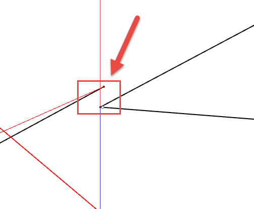
Please check the torsions in nodes: sometimes the members are not connected correctly at the nodal points (minimal inaccuracies) and there are two nodes very close to each other (see the image). This results in unrealistically large torsions about the member axis, which lead to these moments.