
In the Geotechnical Analysis add-on, the Hoek-Brown material model is available. The model shows linear-elastic ideal-plastic material behavior. Its nonlinear strength criterion is the most common failure criterion for stone and rocks.
You can enter the material parameters using
- Rock parameters directly, or alternatively via
- GSI classification.
Detailed information about this material model and the definition of the input in RFEM can be found in the respective chapter Hoek-Brown Model of the online manual for the Geotechnical Analysis add-on.
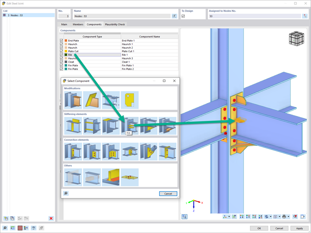
Mit der Komponente "Rippe" können Sie sehr schnell eine beliebige Anzahl an Längsrippen an einem Stabblech definieren. Durch die Vorgabe eines Referenzobjektes lassen sich daran automatisch Schweißnähte vorgeben.
Die Komponente "Rippe" lässt sich auch an kreisförmigen Hohlprofilen anordnen. Dafür wird zusätzlich die Vorgabe der Winkel zwischen den Rippen benötigt.
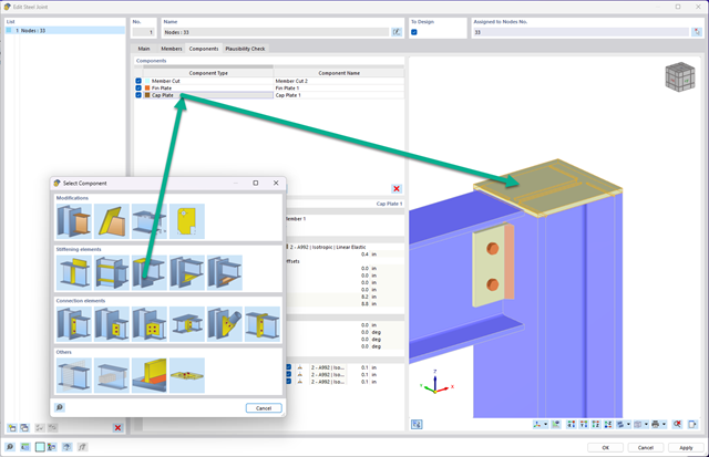
You can now insert a cap plate in steel joints with only a few clicks. You can enter the data using the known definition types "Offsets" or "Dimensions and Position". By specifying a reference member and the cutting plane, it is also possible to omit the Member Section component.
This component allows you to easily model cap plates on column ends, for example.
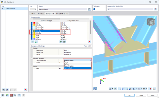
You can use the "Plate Cut" component to cut plates (for example, gusset plates, fin plates, and so on). There are various cutting methods available:
- Plane: The cut is performed on the closest surface to the reference plate.
- Surface: Only the intersecting parts of plates are cut.
- Bounding Box: The outermost dimension consisting of width and height is cut out of the plate as a rectangle.
- Convex Envelope: The outer hull of the cross-section is used for the plate cut. If there are fillets at the corner nodes of the cross-section, the cut is adapted to them.
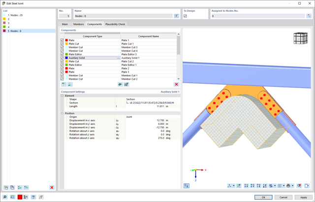
In the Steel Joints add-on, you can perform precise cuts on plates and structural components using the "Auxiliary Solid" component. Within this component, you can use the shapes of a box, a cylinder, or any cross-section as a guide object.
Go to Explanatory Video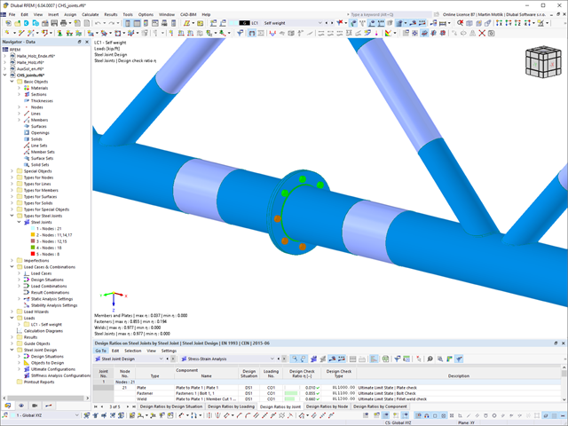
The Steel Joints add-on provides you with the option to connect circular hollow sections using welds.
It is possible to connect the circular sections to each other or to planar structural components. The fillets of standard and thin-walled sections can also be connected with a weld.
Go to Explanatory Video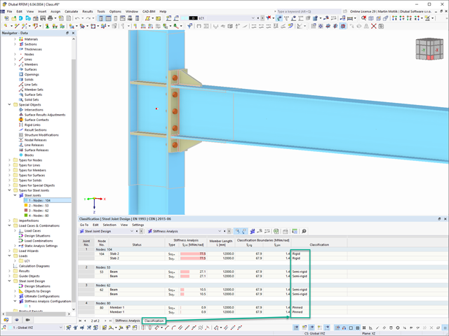
In the Steel Joints add-on, you can classify the joint stiffness.
In addition to the initial stiffness, the table also shows the limit values for hinged and rigid connections for the selected internal forces N, My, and/or Mz. The resulting classification is then displayed in tables as "hinged", "semi-rigid", or "rigid".
Go to Explanatory Video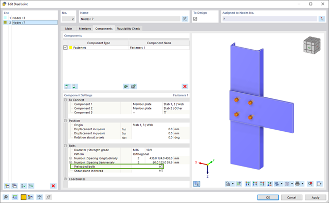
In the Steel Joints add-on, you have this option to consider the preloaded bolts in the calculation of all components.
You can easily activate the prestress using the check box in the bolt parameters, and it has an impact on the stress-strain analysis as well as the stiffness analysis.
Go to Explanatory Video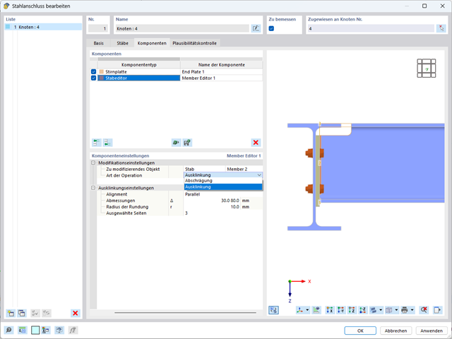
In the Member Editor component, you can also select the entire member as the modifying object instead of the individual member plates. This way, you can apply both operations "Notch" and "Chamfer" to several member plates.
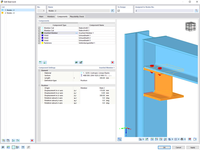
When designing connections, you can now also insert a new member as a component directly in the Steel Joints add-on. This will only be considered for the connection design. You can use the Weld and Fasteners components to connect to other members.
Furthermore, it is possible to use the Member Section and Member Editor components and arrange reinforcement elements on the inserted member, such as stiffeners and tapers.
Go to Explanatory Video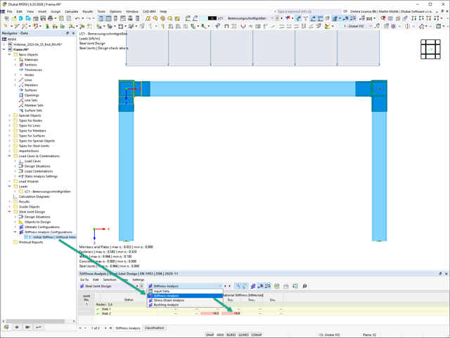
In the Steel Joints add-on, you can determine the initial stiffness Sj,ini according to Eurocode and AISC. This can be done for selected members with reference to the internal forces N, My, and Mz.
In the Members tab of the input dialog box of the Steel Joints add-on, you can select the desired internal forces via a checkbox. Multiple selection is possible. For these internal forces, the stiffness analysis is carried out with a positive and a negative sign.
Go to Explanatory Video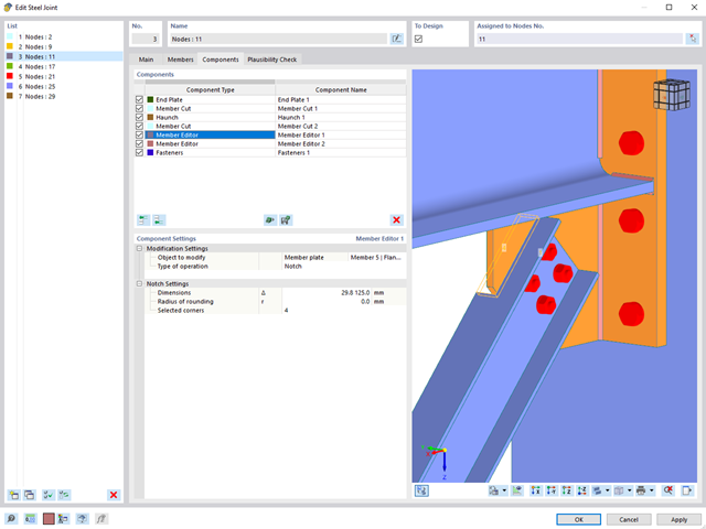
The "Member Editor" component allows you to modify the individual or several member plates in the Steel Joints add-on.
You can use the chamfer, notch, rounding, and hole operations with multiple shapes. It is possible to apply both operations, "Notch" and "Chamfer", for several member plates.
In this way, you can notch flanges from I-sections, for example (see the image).
Go to Explanatory Video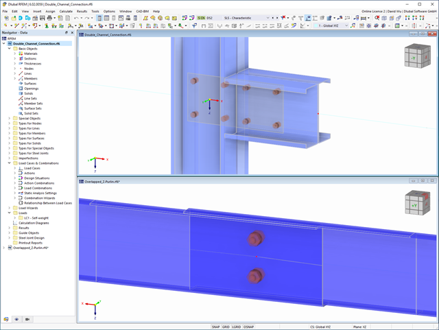
In the Steel Joint add-on, you can design the connections of members with composite cross-sections. Furthermore, you can perform joint design checks for almost all thin-walled cross-sections in the RFEM library.
Go to Explanatory Video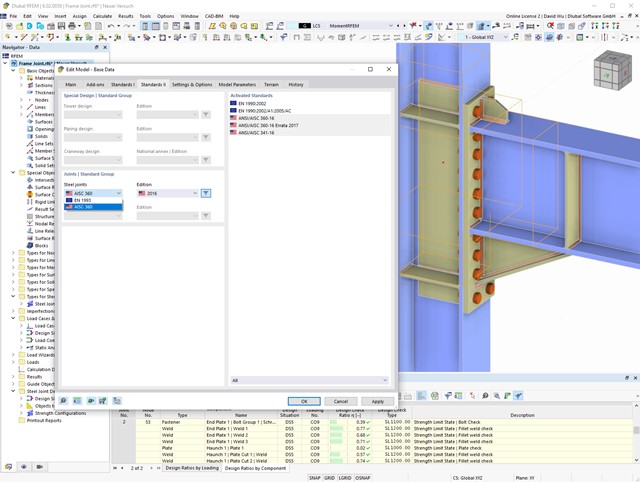
In the Steel Joints add-on, you can design connections according to the American standard ANSI/AISC 360‑16. The following design procedures are integrated:
- Load and Resistance Factor Design (LRFD)
- Allowable Stress Design (ASD)
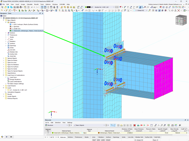
Here, the weld design becomes child's play. Using the specially developed material model "Orthotropic | Plastic | Weld (Surfaces)", you can calculate all stress components plastically. The stress τperpendicular is also considered plastically.
Using this material model you can design welds closer to reality and more efficiently.
Go to Explanatory Video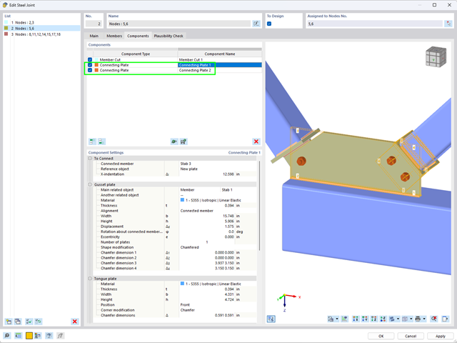
Using the "Connecting Plate" component, you can additionally and automatically create a new gusset plate in the Steel Joints add-on. This saves you separate components, and the other elements, such as a cap plate and a slide plate, are thus automatically taken into account with their dimensions.
Go to Explanatory Video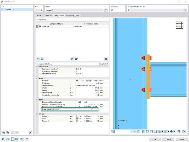
To determine the shear resistance of bolts, you can use the Steel Joints add-on to specify whether there is a shaft or a thread in the shear plane.
Go to Explanatory Video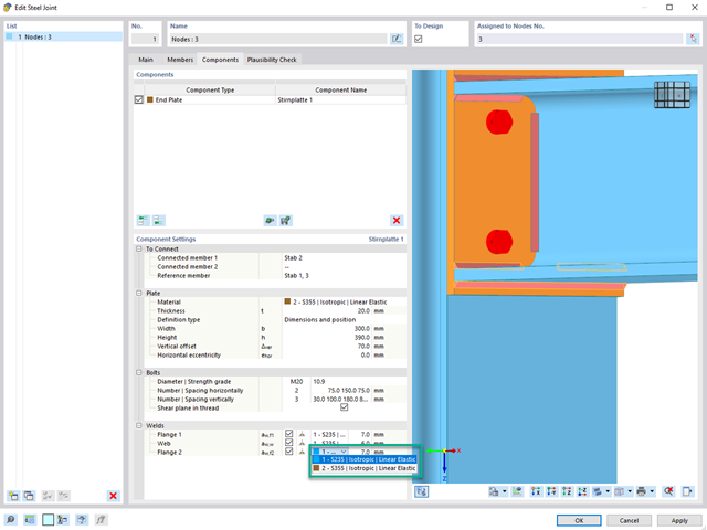
If a weld seam connects two plates with different materials, it is possible to select from a combo box in the Steel Joints add-on which one of both materials should be used for the weld seam.
Go to Explanatory Video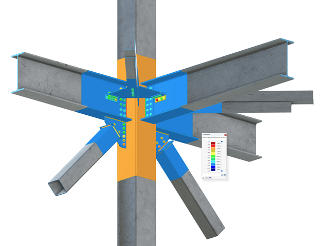
Complex Connection of Horizontal Beams to Column and Connection of Reinforcing Diagonals
The connection model was modeled using about 50 components. The model was created according to the real example of use in structure.
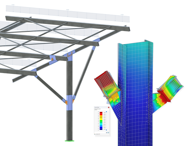
Steel bolted connections with gusset plates on the canopy structure.
Download the structural analysis model and open it with the finite element program RFEM 6 using Steel Joints Add-on.
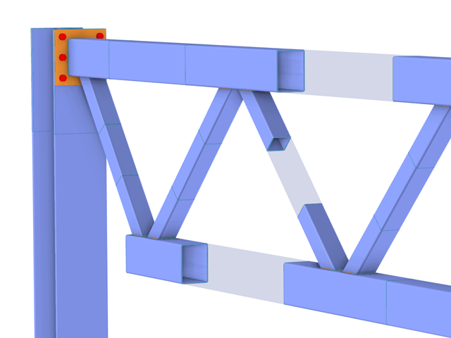
In the case of rectangular cross-sections, you can usually achieve a direct connection by using welds. However, you can also connect them to other cross-sections in the same way. Furthermore, other components such as end plates help you to connect the rectangular cross-sections to other structural components.
.png?mw=640&hash=55038d2a1591f62179796666cb9b2fede0274e19)
A graphical and tabular output of the results for deformations, stresses, and strains helps you when determining the soil solids. To achieve this, use the special filter criteria for targeted selection of results.
The program doesn't leave you alone with the results. If you want to graphically evaluate the results in the soil solids, you can use the guide objects. For example, you can define clipping planes. This allows you to view the corresponding results in any plane of the soil solid.
And not just that. The utilization of result sections and clipping boxes facilitates the precise graphical analysis of the soil solid.
You already know that it is possible to model and analyze a soil and a structure in the entire model. As a result, you have explicitly taken into account the soil-structure interaction. By modifying a component, you achieve the immediate correct consideration in the analysis as well as in the results for the entire system of the soil and structure.

Are you ready for the evaluation? Use the calculation diagrams, which show the distribution of a specific result during the calculation.
You can freely define the layout of the vertical and horizontal axes of the calculation diagram. This allows you, for example, to consider the settlement distribution of a certain node, depending on the load.

Your data are always documented in a multilingual printout report. You can adjust the content at any time and save it as a template. You can also add graphics, texts, MathML formulas, and PDF documents to your report with just a few clicks.
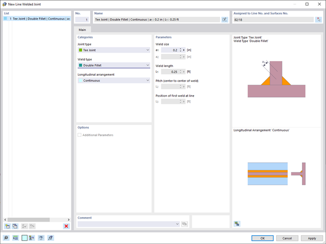
In RFEM 6, it is possible to define line welds between surfaces and to calculate the weld stresses using the Stress-Strain Analysis add-on.
The following joint types are available:
- Butt Joint
- Corner joint
- Lap Joint
- T-joint
Depending on the selected joint type, you can select the following weld types:
- Single Square
- Double Square
- Double Bevel
- Single V
- Double V
- Single U
- Double U
- Single J
- Double J

Enter and model a soil solid directly in RFEM. You can combine the soil material models with all common RFEM add-ons.
This allows you to easily analyze the entire models with a complete representation of the soil-structure interaction.
All parameters required for the calculation are automatically determined from the material data that you have entered. The program then generates the stress-strain curves for each FE element.

Did you know? You can enter the soil layers that you have obtained from the subsoil expertises done in the locations into the program in the form of soil samples. Assign the explored soil materials, including their material properties, to the layers.
For the definition of the samples, you can enter the data in tables as well as in the respective editing dialog box. Furthermore, you can also specify the groundwater level in the soil samples.

The soil solids that you want to analyze are summarized in soil massifs.
Use the soil samples as a basis for a definition of the respective soil massif. This way, the program allows for user-friendly generation of the massif, including the automatic determination of the layer interfaces from the sample data, as well as the groundwater level and the boundary surface supports.
Soil massifs provide you with the option to specify a target FE mesh size independently of the global setting for the rest of the structure. You can thus consider the various requirements of the building and soil in the entire model.

Do you want to model and analyze the behavior of a soil solid? To ensure this, special suitable material models have been implemented in RFEM.
You can use the modified Mohr-Coulomb model with a linear-elastic ideal-plastic model or a nonlinear elastic model with an oedometric stress-strain relation. The limit criterion, which describes the transition from the elastic area to that of the plastic flow, is defined according to Mohr-Coulomb.