
The building model is calculated in two phases:
- Global 3D calculation of the global model, where the slabs are modeled as a rigid plane (diaphragm) or as a bending plate
- Local 2D calculation of the individual floors
After the calculation, the results of the columns and walls from the 3D calculation and the results of the slabs from the 2D calculation are combined in a single model. This means that there is no need to switch between the 3D model and the individual 2D models of the slabs. The user only works with one model, saves valuable time, and avoids possible errors in the manual data exchange between the 3D model and the individual 2D ceiling models.
The vertical surfaces in the model can be divided into shear walls and opening lintels. The program automatically generates internal result members from these wall objects, so they can be designed as members according to any standard in the Concrete Design add-on.

Have you activated the Building Model add-on? Very good! This allows you to display the center of rigidity in tabular and graphical form. Use it for your dynamic analysis, for example.

Are you ready for the evaluation? Use the calculation diagrams, which show the distribution of a specific result during the calculation.
You can freely define the layout of the vertical and horizontal axes of the calculation diagram. This allows you, for example, to consider the settlement distribution of a certain node, depending on the load.

Do you want to model and analyze the behavior of a soil solid? To ensure this, special suitable material models have been implemented in RFEM.
You can use the modified Mohr-Coulomb model with a linear-elastic ideal-plastic model or a nonlinear elastic model with an oedometric stress-strain relation. The limit criterion, which describes the transition from the elastic area to that of the plastic flow, is defined according to Mohr-Coulomb.
.png?mw=640&hash=403c565ab80c4dd45c2d1356634fb74a90428b70)
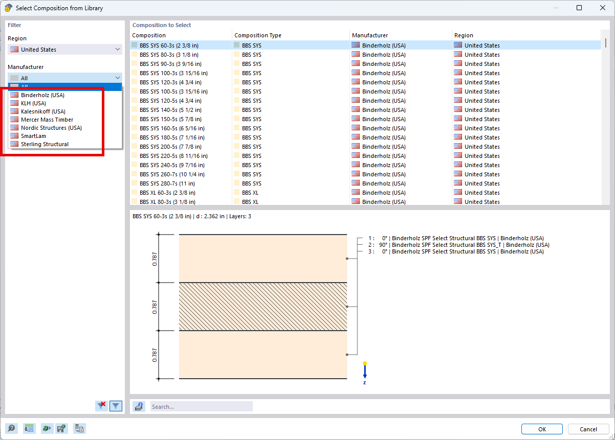
Among others, the following cross-laminated timber manufacturers are available in the layer structure library:
- Binderholz (USA)
- KLH (USA, CAN)
- Kalesnikoff (USA, CAN)
- Nordic Structures (USA, CAN)
- Mercer Mass Timber
- SmartLam
- Sterling Structural
- Superstructures listed in Lignatec Edition 32 "Cross-Laminated Timber of Swiss Production"
By importing a structure from the layer structure library, all relevant parameters are adopted automatically. The library is continually updated.

Compared to the RF‑SOILIN add-on module (RFEM‑5), the following new features have been added to the Geotechnical Analysis add-on for RFEM 6:
- Creation of the layered soil as a 3D model from the entirety of the defined soil samples
- Recognized material law according to Mohr-Coulomb for soil simulation
- Graphical and tabular output of stresses and strains at any depth of the soil
- Optimal consideration of the soil-structure interaction on the basis of an overall model
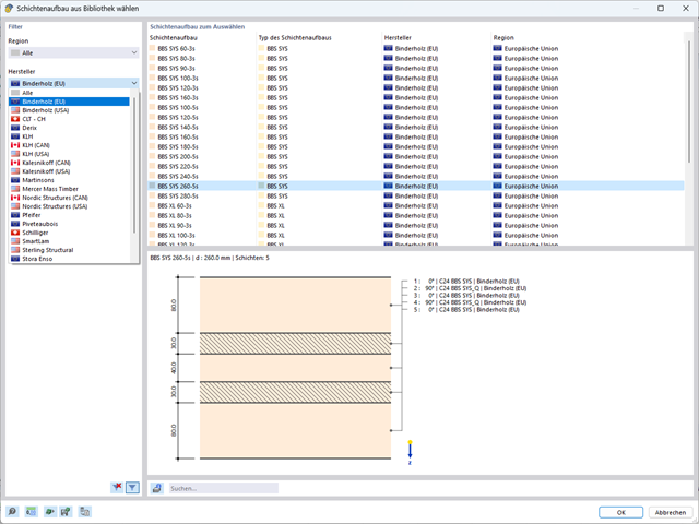
A library for cross-laminated timber panels is implemented in RFEM, from which you can import the manufacturer's layer structures (for example, Binderholz, KLH, Piveteaubois, Södra, Züblin Timber, Schilliger, Stora Enso). In addition to the layer thicknesses and materials, there is also the information about stiffness reductions and the narrow side bonding.
Go to Explanatory Video
The soil solids that you want to analyze are summarized in soil massifs.
Use the soil samples as a basis for a definition of the respective soil massif. This way, the program allows for user-friendly generation of the massif, including the automatic determination of the layer interfaces from the sample data, as well as the groundwater level and the boundary surface supports.
Soil massifs provide you with the option to specify a target FE mesh size independently of the global setting for the rest of the structure. You can thus consider the various requirements of the building and soil in the entire model.

Your data are always documented in a multilingual printout report. You can adjust the content at any time and save it as a template. You can also add graphics, texts, MathML formulas, and PDF documents to your report with just a few clicks.

Using the "Load Transfer Only" story type, you can consider slabs without stiffness effect in and out of the plane in the Building Model add-on. This element type collects the loads on the slab and transfers them to the supporting elements of a 3D model. Thus, you can simulate secondary components, such as grillage and similar load distribution elements, without any further effect in the 3D model.
You already know that it is possible to model and analyze a soil and a structure in the entire model. As a result, you have explicitly taken into account the soil-structure interaction. By modifying a component, you achieve the immediate correct consideration in the analysis as well as in the results for the entire system of the soil and structure.
.png?mw=640&hash=55038d2a1591f62179796666cb9b2fede0274e19)
A graphical and tabular output of the results for deformations, stresses, and strains helps you when determining the soil solids. To achieve this, use the special filter criteria for targeted selection of results.
The program doesn't leave you alone with the results. If you want to graphically evaluate the results in the soil solids, you can use the guide objects. For example, you can define clipping planes. This allows you to view the corresponding results in any plane of the soil solid.
And not just that. The utilization of result sections and clipping boxes facilitates the precise graphical analysis of the soil solid.

Are you afraid that your project will end in the digital tower of Babel? The Building Model add-on for RFEM supports you in your work on a construction project with several stories. It allows you to define a building by means of stories at specified elevations. You can adjust the stories in many ways afterwards and also select the story slab stiffness. Information about the stories and the entire model (center of gravity, center of rigidity) is displayed for you in tables and graphics.
More About Building Model
Several modeling tools are available for elements in building models:
- Vertical line
- Column
- Wall
- Beam
- Rectangular floor
- Polygonal floor
- Rectangular floor opening
- Polygonal floor opening
This feature allows you to define the element on the ground plane (for example, with a background layer) with the associated multiple element creation in space.

Did you know? You can enter the soil layers that you have obtained from the subsoil expertises done in the locations into the program in the form of soil samples. Assign the explored soil materials, including their material properties, to the layers.
For the definition of the samples, you can enter the data in tables as well as in the respective editing dialog box. Furthermore, you can also specify the groundwater level in the soil samples.
Entering soil layers for soil samples is performed in a clearly arranged dialog box. A corresponding graphical representation supports clarity and makes checking the input user-friendly.
An extensible database facilitates the selection of soil material properties. The Mohr-Coulomb model as well as a nonlinear model with stress and strain dependent stiffness are available for a realistic modeling of the soil material behavior.
You can define any number of soil samples and layers. The soil is generated from all entered samples using 3D solids. Assignment to the structure is carried out using coordinates.
The soil body is calculated according to the nonlinear iterative method. The calculated stresses and settlements are displayed graphically and in tables.

The stress and strain results by surface can be output in the surface result table according to the thickness layer.
_ENG.png?mw=640&hash=1053c9bef400e9f5361c9c3278f76a272fcc4ddf)
Have you activated the Time-Dependent Analysis (TDA) add-on? Very well, now you can add time data to load cases. After you have defined the start and end of the load, the influence of creep at the end of the load is taken into account. The program allows you to model creep effects for frame and truss structures made of reinforced concrete.
In this case, the calculation is performed nonlinearly according to the rheological model (Kelvin and Maxwell model).
Was the calculation successful? You can now display the determined internal forces in tables and graphics, and consider them in the design.

Do you have great respect for the ravages of time? After all, it eventually gnaws at your construction projects. Use the Time-Dependent Analysis (TDA) add-on to consider the time-dependent material behavior of members. Long-term effects, such as creep, shrinkage, and aging, can influence the distribution of internal forces, depending on the structure. Prepare for this optimally with this add-on.
More About Time-Dependent Analysis (TDA)
- Consideration and display of story masses
- Listing of structural elements and their information
- Automated creation of result sections on shear walls
- Output of section resultants in global direction for determining shear forces
- Optional definition of rigid diaphragm by story (story modeling)
- Stiffness type Floor Slab - Rigid Diaphragm
- Defining floor sets,
- for example, calculation of slabs as a 2D position within the 3D model
- Shear walls: Automatic definition of result members with any cross-section
- Design of rectangular cross-sections using the Concrete Design add-on
- Definition of deep beams
- Design with the Concrete Design add-on
- Tabular output of story actions, interstory drift, and center points of mass and stiffness, as well as the forces in shear walls
- Separate result display of the floor and stiffening design
- Optional neglecting of openings of a certain size