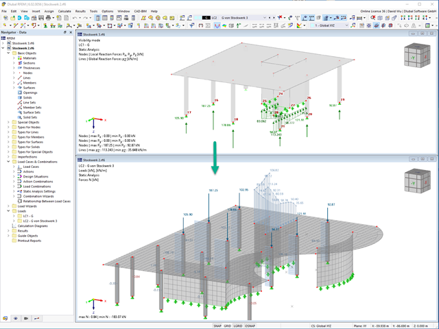
This function provides you with the option to adopt reaction forces from other models as nodal and line loads.
The option not only transfers the reaction load as an action, but digitally couples the support load of the original model with the load size of the target object. The subsequent changes in the original model are automatically adopted in the target model.
This technology supports the concept of positional statics and allows you to digitally connect the individual positions of the same Dlubal Center project.
Go to Explanatory Video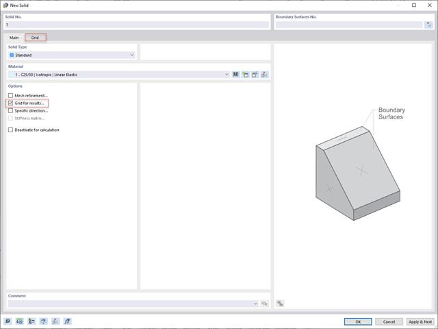
In addition to the "Mesh Refinement" and "Specific Direction" options for solids, you can also activate the "Grid for Results" option, which allows for organizing grid points in the solid space. Among other things, the center of gravity can be set as the origin. There is also the option to activate or deactivate the visibility of the grid for numerical results in "Navigator – Display" under Basic Objects.

Did you know? In contrast to other material models, the stress-strain diagram for this material model is not antimetric to the origin. You can use this material model to simulate the behavior of steel fiber-reinforced concrete, for example. Find detailed information about modeling steel fiber-reinforced concrete in the technical article about Determining the material properties of steel-fiber-reinforced concrete.
In this material model, the isotropic stiffness is reduced with a scalar damage parameter. This damage parameter is determined from the stress curve defined in the Diagram. The direction of the principal stresses is not taken into account. Rather, the damage occurs in the direction of the equivalent strain, which also covers the third direction perpendicular to the plane. The tension and compression area of the stress tensor is treated separately. In this case, different damage parameters apply.
The "Reference element size" controls how the strain in the crack area is scaled to the length of the element. With the default value zero, no scaling is performed. Thus, the material behavior of the steel fiber concrete is modeled realistically.
Find more information about the theoretical background of the "Isotropic Damage" material model in the technical article describing the Nonlinear Material Model Damage.
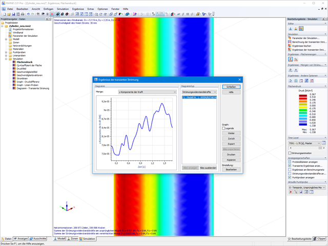
By solving the numerical flow problem, you can obtain the following results on and around the model:
- Pressure on structure surface
- Coefficient Cp distribution on the structure surfaces
- Pressure field about the structure geometry
- Velocity field about the structure geometry
- Turbulence k-ω field about the structure geometry
- Turbulence k-ε field about the structure geometry
- Velocity vectors about the structure geometry
- Streamlines about the structure geometry
- Forces on member-shaped structures that were originally generated from member elements
- Convergence diagram
- Direction and size of the flow resistance of the defined structures
Despite this amount of information, RWIND 2 remains clearly arranged, as is typical for the Dlubal programs. You can specify freely definable zones for a graphic evaluation. Voluminously displayed flow results about the structure geometry are often confusing – you know the problem for sure. That's why RWIND Basic provides freely movable section planes for the separate display of the "solid results" in a plane. For the 3D branched streamline result, you have an option to select between a static and an animated display in the form of moving line segments or particles. This option helps you to represent the wind flow as a dynamic effect.
You can export all results as a picture or, especially for the animated results, as a video.
Always keep an eye on your results. In addition to the resulting load cases in RFEM or RSTAB (see below), the results from the aerodynamics analysis in RWIND 2 represent the flow problem as a whole:
- Pressure on structure surface
- Pressure field about structure geometry
- Velocity field about structure geometry
- Velocity vectors about structure geometry
- Flow lines about structure geometry
- Forces on member-shaped structures that were originally generated from member elements
- Convergence diagram
- Direction and size of the flow resistance of the defined structures
These results are displayed in the RWIND 2 environment and evaluated graphically. The flow results around the structure geometry in the overall display are rather confusing, but the program has a solution for this. In order to present clearly arranged results, freely movable section planes are displayed for the separate display of the 'solid results' in a plane. Accordingly, for the 3D branched streamline result, the program presents you an animated display in the form of moving lines or particles in addition to the static one. This option helps to represent the wind flow as a dynamic effect.
You can export all results as a picture or, especially for the animated results, as a video.
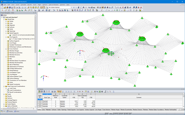
The results of the form‑finding process are a new shape and corresponding inner forces. The usual results, such as deformations, forces, stresses, and others can be displayed in the RF‑FORM‑FINDING case.
This prestressed shape is available as the initial state for all other load cases and combinations in the structural analysis.
For more ease when defining load cases, the NURBS transformation can be used (Calculation Parameters/Form-Finding). This feature moves the original surfaces and cables into position after form‑finding.
By using the grid points of surfaces or the definition nodes of NURBS surfaces, free loads can be situated on selected parts of the structure.