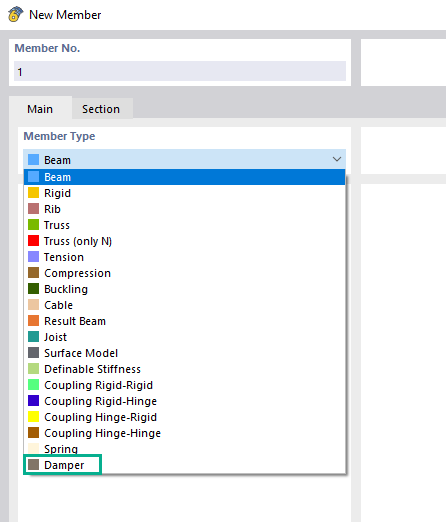
Using the "Damper" member type, you can define a damping coefficient, a spring constant, and a mass. This member type extends the possibilities within the Time History Analysis.
With regard to viscoelasticity, the "Damper" member type is similar to the Kelvin-Voigt model, which consists of the damping element and an elastic spring (both connected in parallel).

The building model is calculated in two phases:
- Global 3D calculation of the global model, where the slabs are modeled as a rigid plane (diaphragm) or as a bending plate
- Local 2D calculation of the individual floors
After the calculation, the results of the columns and walls from the 3D calculation and the results of the slabs from the 2D calculation are combined in a single model. This means that there is no need to switch between the 3D model and the individual 2D models of the slabs. The user only works with one model, saves valuable time, and avoids possible errors in the manual data exchange between the 3D model and the individual 2D ceiling models.
The vertical surfaces in the model can be divided into shear walls and opening lintels. The program automatically generates internal result members from these wall objects, so they can be designed as members according to any standard in the Concrete Design add-on.
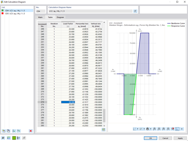
For calculation diagrams, the "2D | Hinge" is available. These hinge diagrams show the hinge response of load situations for nonlinear hinges.
For calculations with several load situations, such as is the case with pushover analyzes and time history analysis, you can evaluate the state of the hinge in each load step.
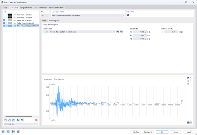
The Time History Analysis add-on provides you with accelerograms for the calculation. This extension allows for dynamic structural analysis of the acceleration-time diagrams.
There is an extensive library of earthquake records available for you, but you can also enter or import your own diagrams. The time history analysis is performed using the modal analysis or the linear implicit Newmark analysis.
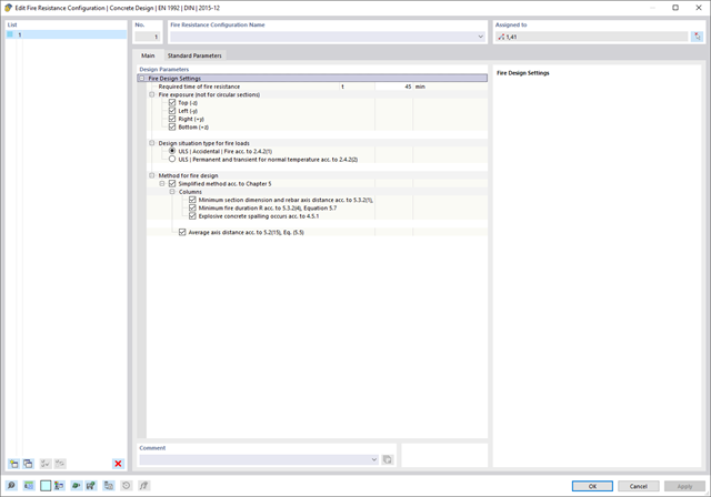
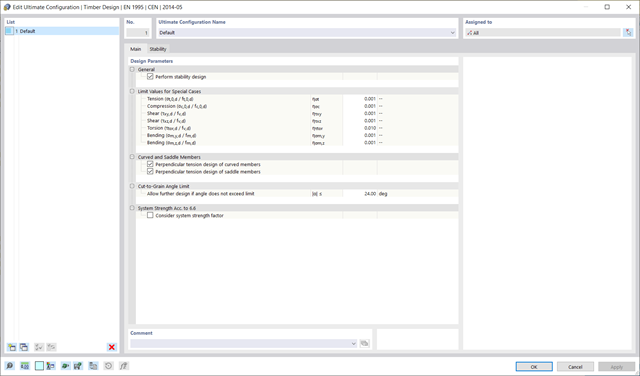
The Concrete Design add-on provides you with the option to perform the simplified fire resistance design according to EN 1992‑1‑2 for columns (Section 5.3.2) and beams (Section 5.6).
The following design checks are available for the simplified fire resistance design:
- Columns: Minimum cross-sectional dimensions for rectangular and circular sections according to Table 5.2a as well as Equation 5.7 for calculating time of fire exposure
- Beams: Minimum dimensions and center distances according to Table 5.5 and Table 5.6
You can determine the internal forces for the fire resistance design according to two methods.
- 1 Here, the internal forces of the accidental design situation are included directly into the design.
- 2 The internal forces of the design at normal temperature are reduced by the factor Eta,fi (ηfi), then used in the fire resistance design.
Furthermore, it is possible to modify the axis distance according to Eq. 5.5.
- Analysis of time diagrams and accelerograms (acceleration-time diagrams exciting the supports of a structure)
- Combination of user-defined time diagrams with nodal, member, and surface loads, as well as free and generated loads
- Combination of several independent excitation functions
- Linear implicit Newmark analysis or modal analysis in time history
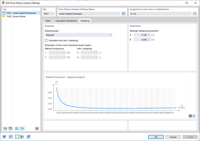
- Structural damping using Raleigh damping coefficients or Lehr's damping value
- Graphical display of results in calculation diagrams
- Result display in individual time steps or as an envelope during the entire time period
- Extensive library of seismic events (accelerograms)
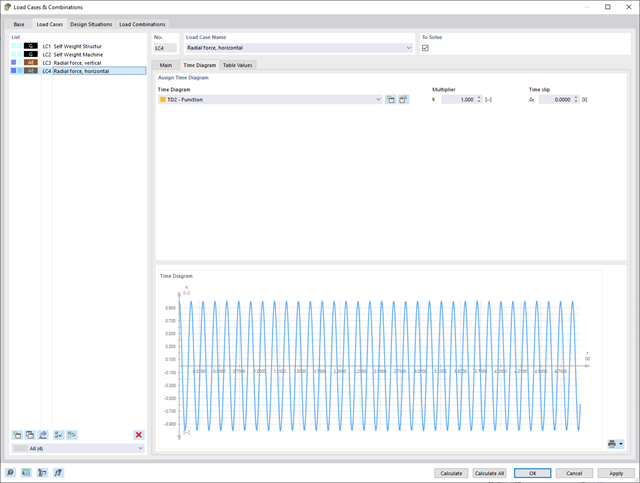
It is necessary to enter the required force-time diagrams. They can be combined in load cases or load combinations of the type Time History Analysis | Time Diagrams with the loading in order to define where and in which direction the force-time diagrams act.
The second option is to enter acceleration-time diagrams, which can be used in the load cases of the Time History Analysis | Accelerogram type.
All calculation parameters are specified in the time history analysis settings. These include, for example, the type of analysis method and the maximum calculation time.
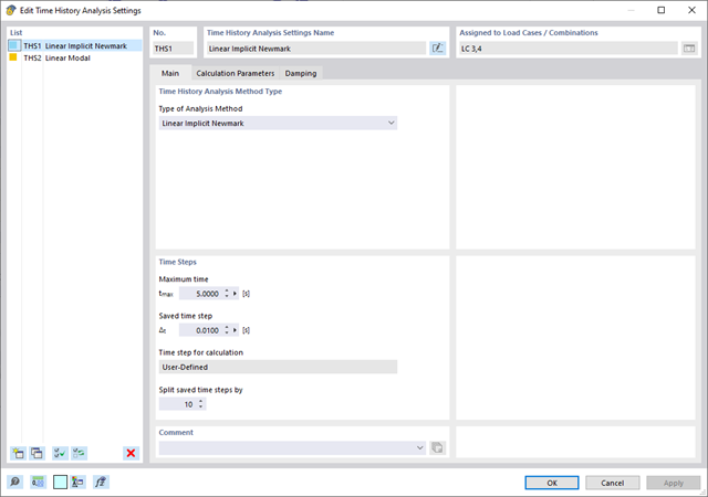
The time history analysis is performed with the modal analysis or the linear implicit Newmark analysis. The time history analysis in this add-on is limited to linear structural systems. Although the modal analysis represents a fast algorithm, it is necessary to use a certain number of eigenvalues to ensure the required accuracy of results.
The implicit Newmark analysis is a very precise method, independent of the number of eigenvalues used, but requires sufficient small time steps for the calculation.
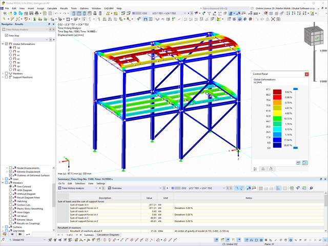
As soon as the program has completed the calculation, the summary of the results is listed. All result windows are integrated in the main program RFEM/RSTAB. You will find all the results arranged in tables; they can be displayed for each individual time step or as an envelope, and you also have the option of displaying the results graphically as well as animating them.
The results from the time history analysis can be displayed in the calculation diagrams. All the results are shown as a function of time. You can export the numeric values to MS Excel.
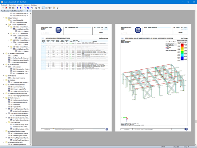
All result tables and graphics are part of the RFEM/RSTAB printout report. In this way, you can ensure clearly arranged documentation. You can also export the tables to MS Excel.
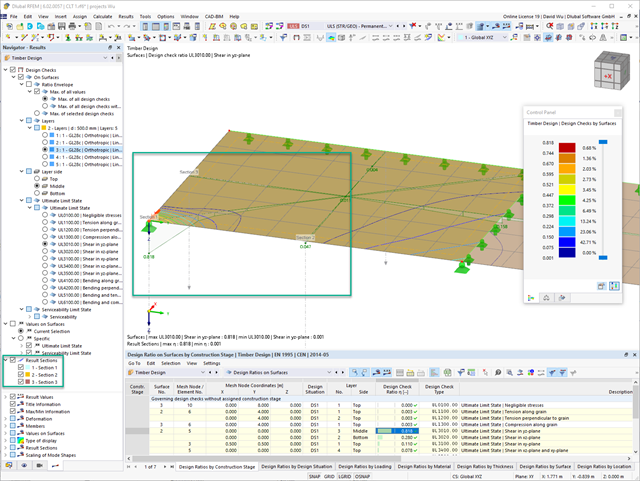
You can graphically evaluate result sections for the timber surface design. This can be done in the RFEM graphic as well as in the result history window. The sections can be placed at any location in order to evaluate the design results in detail.
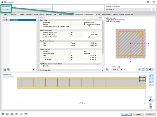
Utilize this time-saving step! This feature allows you to define or edit the member reinforcement for several members or member sets at the same time.
Go to Explanatory Video
Your data are always documented in a multilingual printout report. You can adjust the content at any time and save it as a template. You can also add graphics, texts, MathML formulas, and PDF documents to your report with just a few clicks.

Note that the definition of the effective lengths in the Aluminum Design add-on is an essential requirement for the stability analysis. For this, define the nodal supports and effective length factors in the input dialog box. Do you want to clearly document the nodal supports and the resulting segments with the associated effective length factors? To check the input data, it is best for you to use the graphic display in the RFEM/RSTAB work window. Thus, you can comprehend the design at any time with minimum effort.
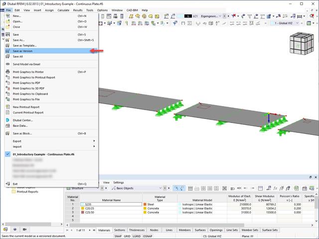
It is possible to save different model versions within a model by using the Save as Version function. In the Base Data of the model, the different model versions can be displayed in the History tab.
- Arbitrary definition of the charring time
- Option to calculate with or without adhesion of the layer for surface structures (cross-laminated timber)
- Free user-defined specification of the fire parameters
- Consideration of Different Effective Lengths in Fire Resistance Design
- Optional design "Compression perpendicular to grain"
- Graphical result display integrated in RFEM/RSTAB, such as a design ratio
- Complete integration of the results into the RFEM/RSTAB printout report
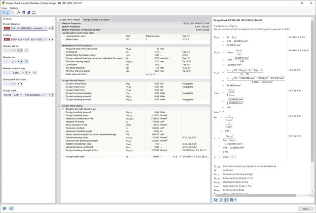
As you probably know, the design checks for the selected members are carried out, taking into account the defined charring time. All necessary reduction factors and coefficients are stored accordingly in the program and are taken into account when determining the load-bearing capacity. That saves you a lot of work.
The effective lengths for the equivalent member design are taken directly from the strength entries. You do not have to enter them again.
After completing the design, the program presents the fire resistance design checks clearly and with all result details. This allows you to follow the results completely transparently. The results also contain all the required parameters, so you can determine the component temperature at the design time.
In addition to all these features, the program allows you to integrate all result tables and graphics, including the ultimate and serviceability limit state results,into the global printout report of RFEM/RSTAB as a part of the steel design results.
You can enter the structural system and calculate the internal forces in the programs RFEM and RSTAB. You have full access to the extensive material and cross-section libraries.
Timber Design is completely integrated into the main programs. At the same time, it automatically takes into account the structure and the available calculation results. You can assign further entries for the timber design, such as effective lengths, cross-section reductions, or design parameters, to the objects to be designed. You can easily select the elements graphically using the [Select] function at many places of the program.
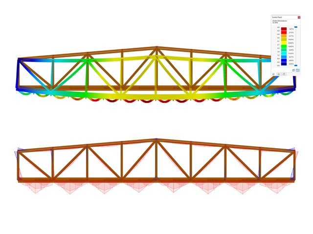
- Calculation of deflections and comparison with the normative or manually adjusted limit values
- Consideration of a precamber for the deflection analysis
- Different limit values are possible, depending on the design situation type
- Manual adjustment of reference lengths and segmentation by direction
- Calculation of deflections related to the initial structure or to the deformed structure
- Automatic consideration of time-dependent deformations by increasing the load with the creep factor (can also be user-defined on the stiffness side)
- Simplified vibration design
- Graphical result display integrated in RFEM/RSTAB; for example, the design ratio of a limit value, the deformation, or the sag
- Complete integration of the results into the RFEM/RSTAB printout report
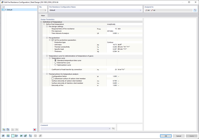
- Manual specification of critical component temperature or automatic determination of component temperature for desired duration
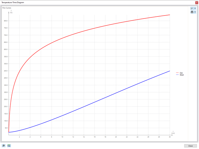
- A wide range of fire curves: standard temperature-time curve, external fire curve, hydrocarbon curve
- Manual adjustment of the essential coefficients for the determination of the steel temperature
- Consideration of hot-dip galvanizing of structural components for the determination of the steel temperature
- Results of a temperature-time diagram for the gas and steel temperature
- Fire protection cladding as a contour or a box cladding with temperature-independent materials can be considered when determining the temperature
- Design of members made of carbon steel or stainless steel
- Cross-section design checks and stability analyses (equivalent member method) according to EN 1993‑1‑2, Clause 4.2.3
- Design checks of the cross-sections of Class 4 according to EN 1993‑1‑2, Annex E.
The structural analysis programs RFEM/RSTAB offer you a wide range of automated functions that make your dayily work easier. One of them is the automatic generation of load and result combinations for the accidental design situation of fire design. The members to be designed with the corresponding internal forces are imported directly from RFEM/RSTAB. You don't need to do anything else. The program has also already stored all information about the material and cross-section for you.
By assigning a fire resistance configuration to the members to be designed, you define the parameters relevant for the fire resistance design. Here you can manually specify the critical steel temperature at the design time. Or let the program to determine the temperature determined automatically for a specified fire duration. You can select from various fire temperature curves and fire protection measures. It is also possible to make further detailed settings, such as the definition of the fire exposure on all sides or three sides
After completing the design, the Dlubal Software presents the fire resistance design checks clearly and with all result details. This makes the results comprehensible in detail. Furthermore, the results also contain all the parameters required for the determination of the component temperature at the design time.
You can also specifically evaluate the temperature distribution in the structural component using the temperature-time diagram.
All result tables and graphics, including the ultimate and serviceability limit state results, can be integrated into the global printout report of RFEM/RSTAB as a part of the steel design results.
Perform the fire resistance design with a reduced load-bearing capacity according to the component temperature determined automatically right at the design time. You can determine this automatically according to various temperature curves in the program (a standard temperature-time curve, an external fire curve, a hydrocarbon curve). For other types of temperature determination, it is also possible for you to manually specify the temperature to be applied in the design. You can determine this, for example, according to the parametric temperature-time curve from DIN EN 1991‑1‑2 or from a fire protection report.
The component temperature to be applied at the design time is determined automatically. You can adjust the coefficients used to determine the temperature. In this step, it is best for you to also select the hot-dip galvanizing. According to the DASt Guideline 027 "Determination of Component Temperature of Hot-Dip Galvanized Steel Components in Case of Fire", a lower emissivity of the steel surface is applied up to a limit temperature. Overall, this gives you a lower temperature for the thus more favorable fire resistance design.
The governing component temperature at the time of analysis can be determined for the fire resistance design automatically using the input. In this case, you can follow the temperature curve in detail as a function of timeby displaying the temperature-time diagram.

Did you know? In contrast to other material models, the stress-strain diagram for this material model is not antimetric to the origin. You can use this material model to simulate the behavior of steel fiber-reinforced concrete, for example. Find detailed information about modeling steel fiber-reinforced concrete in the technical article about Determining the material properties of steel-fiber-reinforced concrete.
In this material model, the isotropic stiffness is reduced with a scalar damage parameter. This damage parameter is determined from the stress curve defined in the Diagram. The direction of the principal stresses is not taken into account. Rather, the damage occurs in the direction of the equivalent strain, which also covers the third direction perpendicular to the plane. The tension and compression area of the stress tensor is treated separately. In this case, different damage parameters apply.
The "Reference element size" controls how the strain in the crack area is scaled to the length of the element. With the default value zero, no scaling is performed. Thus, the material behavior of the steel fiber concrete is modeled realistically.
Find more information about the theoretical background of the "Isotropic Damage" material model in the technical article describing the Nonlinear Material Model Damage.
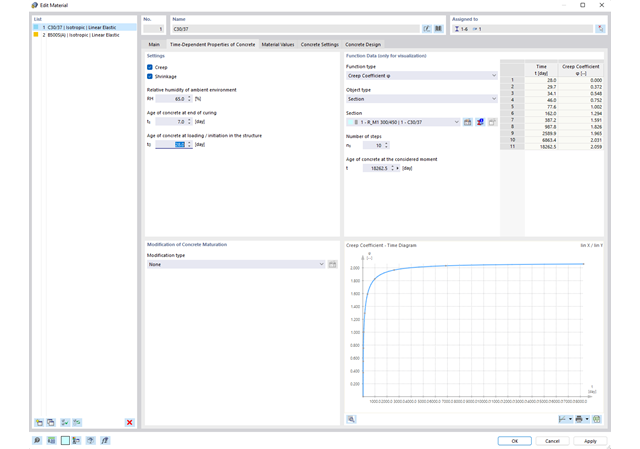
Time-dependent concrete properties, such as creep and shrinkage, are very important for your calculation. You can define them directly for the material in the structural analysis program. In the input dialog box, the time course of the creep or shrinkage function is displayed to you graphically. You can easily select the modification of the applied concrete age, for example, due to a temperature treatment.
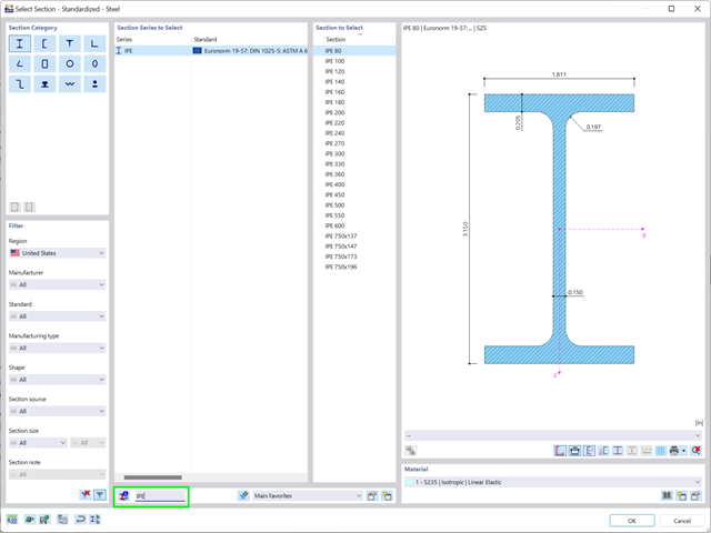
Save your time in the cross-section library and use a short text search to quickly find a desired cross-section or cross-section series.

Do you have great respect for the ravages of time? After all, it eventually gnaws at your construction projects. Use the Time-Dependent Analysis (TDA) add-on to consider the time-dependent material behavior of members. Long-term effects, such as creep, shrinkage, and aging, can influence the distribution of internal forces, depending on the structure. Prepare for this optimally with this add-on.
More About Time-Dependent Analysis (TDA)- Calculation of transient incompressible turbulent wind flow with the BlueDyMSolver solver
- LES SpalartAllmarasDDES turbulence model
- Consideration of stationary solution as initial state for transient calculation
- Automatic determination of analysis period and time steps
- Use of intermediate results during the calculation
- Organized display of time-varying results via time step units
- Diagram of drag force and point probe results over analysis time
- Display of line probe results for any time steps in a diagram
- Freely adjustable wind permeability for surfaces (Go to Product Feature)
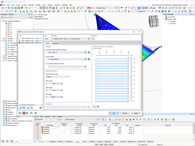
To model structures in RWIND Basic, you find a special application in RFEM and RSTAB. Here, you define the wind directions to be analyzed by means of related angular positions about the vertical model axis. At the same time, you define the elevation-dependent wind profile on the basis of a wind standard. In addition to these specifications, you can use the stored calculation parameters to determine your own load cases for a stationary calculation per each angular position.
As an alternative, you can also use the RWIND Basic program manually, without the interface application in RFEM or RSTAB. In this case, RWIND Basic models the structures and terrain environment directly from the imported VTP, STL, OBJ, and IFC files. You can define the height-dependent wind load and other fluid-mechanical data directly in RWIND Basic.