Determination of Bilinearization for Pushover Curve (N2 Method)

There are various methods available for simplifying the pushover curve. In general, however, they are always carried out using an energy equivalent analysis. In such an analysis, area components are compared with each other.

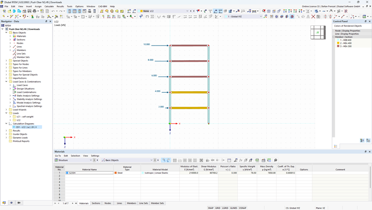
In this article, a two-hinged frame with several stories is selected and plastic hinges are applied. Thus, it is possible to calculate a capacity curve with the Structure Stability add-on.

In the present case, it is necessary to determine the initial stiffness of the idealized system when calculating the idealized elastic-plastic force-displacement relation, so that the areas under both the real and the idealized force-displacement curve are equal.

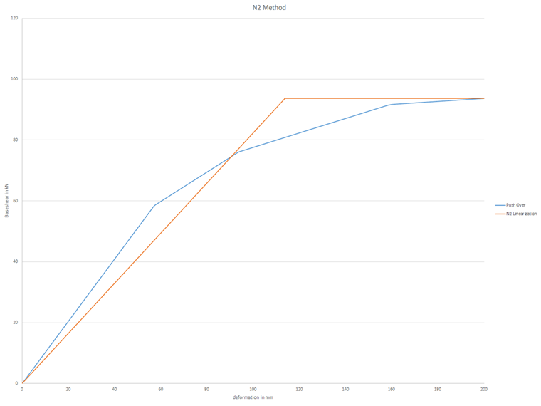
According to the N 2 method, the idealization starts with a linear branch and then turns into a constant horizontal branch. This represents the ideal plastic behavior of the structure.

The simplification is necessary in order to apply the design procedure for the push-over method subsequently. Based on this assumption, the yield displacement of the idealized single degree of freedom system arises.

In order to compare the areas, it is necessary to copy the capacity curve from the structural analysis program to Microsoft Excel. This way, you get the data for load steps or horizontal shear, and the deformation for each load step shown in a table.

In the next step, the maximum deformation and the corresponding horizontal shear are determined. It is almost constant in the last iterations because the maximum load is reached. The corresponding deformation increases in each further iteration. Therefore, it is recommended to choose a step where the deformation change is not so high, so that you reach a sufficient safety, and the failure is still at the beginning of the plastic area. The value pair determined here is now the start value for the bilinearization of the capacity curve.

Taking into account the first point, you can now define a horizontal straight line, which represents the upper part of the bilinearization.

The linearly increasing branch at the beginning of the diagram is also represented by a straight line with a non-zero slope. Now, you vary the slope of this straight line until the enclosed areas are the same. In an Excel spreadsheet, you can do this by means of an iterative determination by increasing the load steps. In the end, you look at the iteration for which both area components are approximately equal. In this way, you can in fact see dy* directly in the table, and you can proceed with further design.

With the help of this calculation, which is described only by a graphic in the Eurocode standard, you can clearly see that a certain amount of effort is required to create the bilinearization. This is only meant to illustrate the cost of time. Because all programs, that have implemented the pushover analysis, usually do it fully automatically, and you do not have to take care of it in detail.

How to transfer the results of the calculation using RFEM or RSTAB to the Excel tool is described in the video on the topf left of this article.