


Theoretical Background
The constrained modulus method represents the interaction between the foundation plate and the soil through an iterative coupling of contact pressures, settlements, and foundation parameters.
The process begins with foundation parameters used to perform an initial FE calculation to determine the distribution of contact pressures. Subsequently, the settlements are calculated in the elastic half-space according to Boussinesq, with the stresses integrated by layer. From this, updated vertical and shear-effective foundation parameters are derived, for which a further FE calculation is performed. The iteration is repeated until the changes in settlements and stresses fall below the convergence threshold.
The online manual for the Geotechnical Analysis add-on provides further information on this topic:
Subject of Analysis
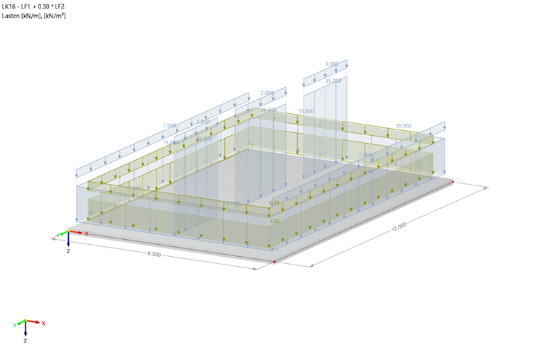
For the displayed foundation slab, the structural analysis—taking into account soil-structure interaction—is to be performed using the constrained modulus method.
Soil Modeling
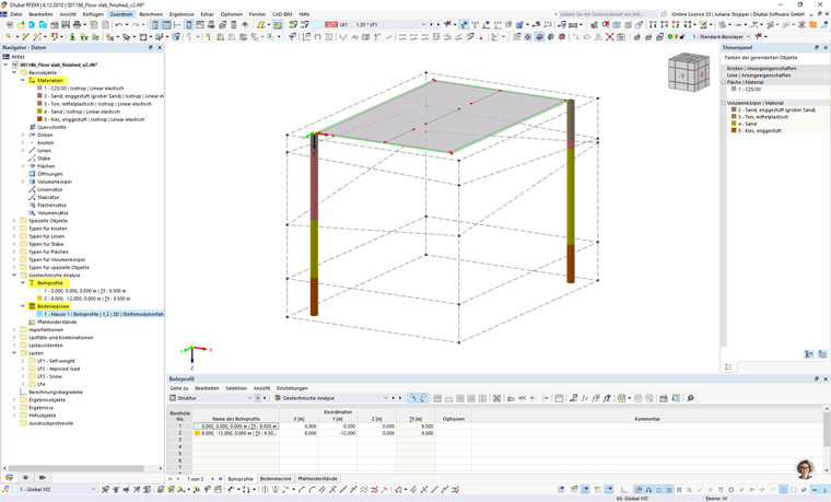
The soil structure is defined in the following steps
- Creating soil materials based on library materials
- Describing the soil structure using boreholes
- Creating the soil mass.
The following series of images briefly summarizes the process. A detailed description of the procedure can be found in the technical article KB 1699 | Creating Soil Masses from Soil Samples in RFEM 6:
1. Constrained Modulus Method as Soil Model Type
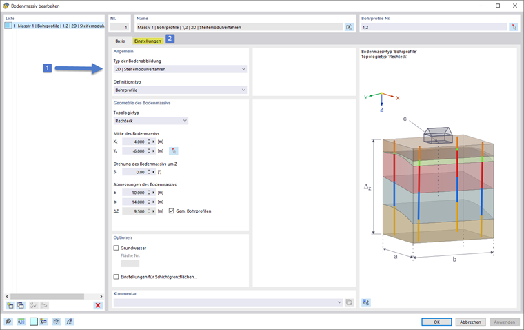
The soil massif serves as the basis for applying the constrained modulus method.
In the “Soil Model Type” text box of the soil massif, you can then select the numerical method for soil modeling.
Select the constrained modulus method (1) from the drop-down menu.
An additional “Settings” section (2) appears, which contains further settings and options.
2. Surface(s) to Support
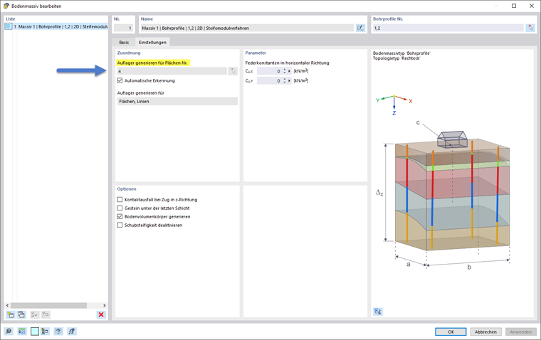
In the settings for the constrained modulus method, you can specify which surfaces are to be supported. In this example, the default settings are used for the remaining options.
Confirm the entry by clicking “OK.” The floor structure is now fully modeled.
3. Generated Support
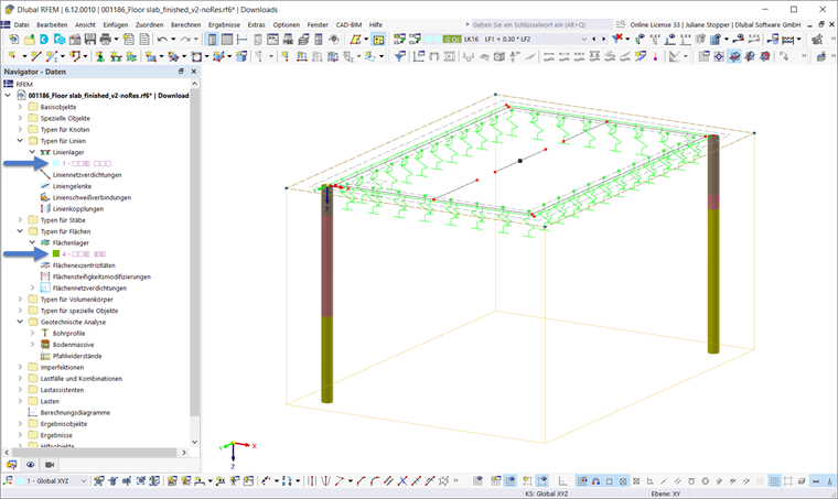
The constrained modulus method generates surface supports as well as line supports along the boundary lines.
The created supports are listed under the types for surfaces and lines, respectively, and are graphically displayed on the model. The support coefficients are determined during the structural analysis.
Analysis
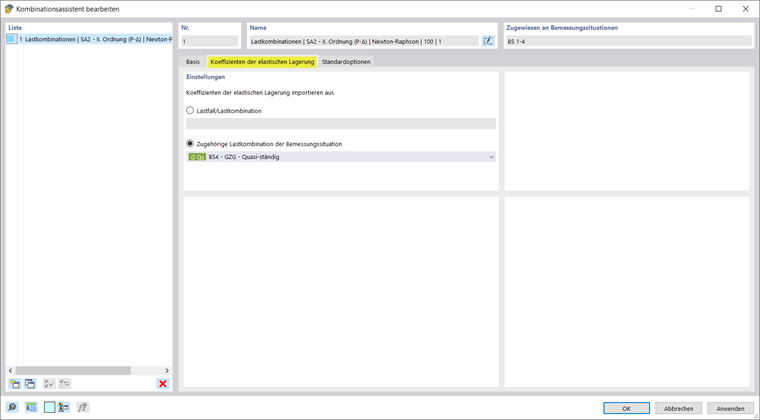
In this example, the load combinations are to be generated by the wizard so that the constrained modulus method is performed for each combination of the quasi-permanent design situation.
For all other design situations, the support conditions are to be adopted from the corresponding quasi-permanent combination.
This is configured accordingly in the combination wizard, as shown in the following series of images.
The generated support combinations are illustrated in the following series of images.
The constrained modulus method is active for all load combinations of the quasi-permanent situation. For all combinations of the remaining design situations, however, the option to perform the transfer of support conditions from the corresponding quasi-permanent load combination has been disabled. For these, a structural analysis is performed without the constrained modulus method.
The model can now be calculated.
Results
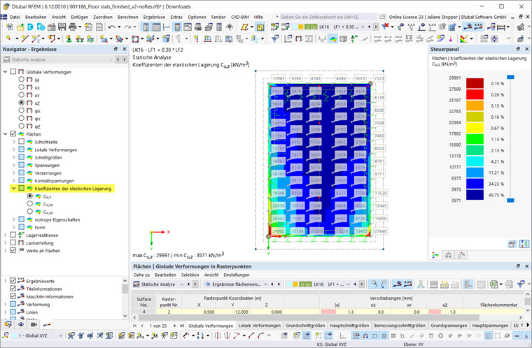
After the structural analysis, the “Coefficients of Elastic Support” result can be selected in the Results navigator for the surfaces, so that the determined foundation properties Cu,z, Cvx,z, and Cv,yz are displayed graphically, as shown in the following image.
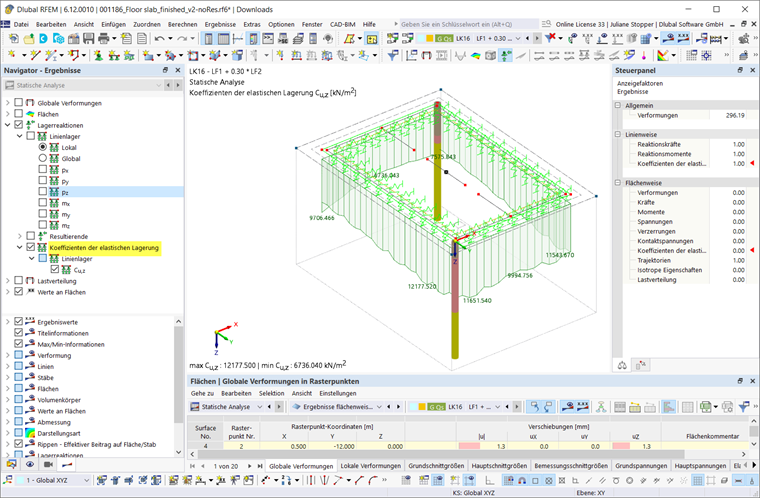
Furthermore, under “Support Reactions,” you can select the result for the “Coefficients of Elastic Support” for the line supports and thus display it in the graph.
Conclusion
Using the constrained modulus method, it is possible to easily consider the soil-structure interaction, thereby significantly improving the accuracy of the finite element analysis results compared to the constant elastic surface foundation.