
Are you ready for the evaluation? Use the calculation diagrams, which show the distribution of a specific result during the calculation.
You can freely define the layout of the vertical and horizontal axes of the calculation diagram. This allows you, for example, to consider the settlement distribution of a certain node, depending on the load.

Do you want to model and analyze the behavior of a soil solid? To ensure this, special suitable material models have been implemented in RFEM.
You can use the modified Mohr-Coulomb model with a linear-elastic ideal-plastic model or a nonlinear elastic model with an oedometric stress-strain relation. The limit criterion, which describes the transition from the elastic area to that of the plastic flow, is defined according to Mohr-Coulomb.
.png?mw=640&hash=403c565ab80c4dd45c2d1356634fb74a90428b70)
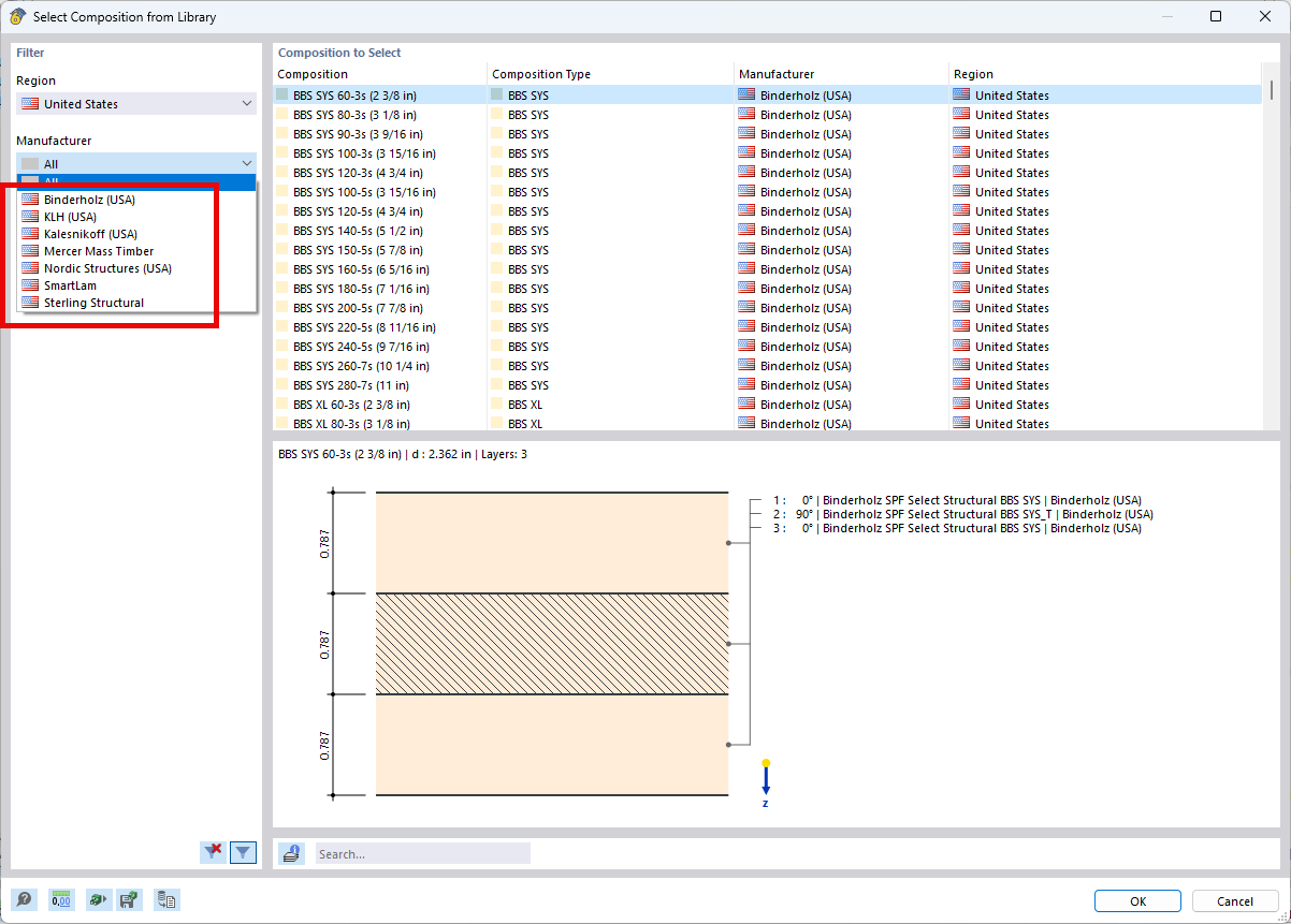
Among others, the following cross-laminated timber manufacturers are available in the layer structure library:
- Binderholz (USA)
- KLH (USA, CAN)
- Kalesnikoff (USA, CAN)
- Nordic Structures (USA, CAN)
- Mercer Mass Timber
- SmartLam
- Sterling Structural
- Superstructures listed in Lignatec Edition 32 "Cross-Laminated Timber of Swiss Production"
By importing a structure from the layer structure library, all relevant parameters are adopted automatically. The library is continually updated.

Compared to the RF‑SOILIN add-on module (RFEM‑5), the following new features have been added to the Geotechnical Analysis add-on for RFEM 6:
- Creation of the layered soil as a 3D model from the entirety of the defined soil samples
- Recognized material law according to Mohr-Coulomb for soil simulation
- Graphical and tabular output of stresses and strains at any depth of the soil
- Optimal consideration of the soil-structure interaction on the basis of an overall model

The Concrete Design add-on allows you to perform the seismic design of reinforced concrete members according to EC 8. This includes, among other things, the following functionalities:
- Seismic design configurations
- Differentiation of the ductility classes DCL, DCM, DCH
- Option to transfer the behavior factor from a dynamic analysis
- Check of the limit value for the behavior factor
- Capacity design checks of "Strong column - weak beam"
- Detailing and particular rules for curvature ductility factor
- Detailing and particular rules for local ductility
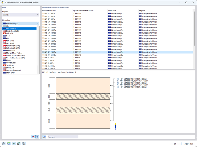
A library for cross-laminated timber panels is implemented in RFEM, from which you can import the manufacturer's layer structures (for example, Binderholz, KLH, Piveteaubois, Södra, Züblin Timber, Schilliger, Stora Enso). In addition to the layer thicknesses and materials, there is also the information about stiffness reductions and the narrow side bonding.
Go to Explanatory Video
The soil solids that you want to analyze are summarized in soil massifs.
Use the soil samples as a basis for a definition of the respective soil massif. This way, the program allows for user-friendly generation of the massif, including the automatic determination of the layer interfaces from the sample data, as well as the groundwater level and the boundary surface supports.
Soil massifs provide you with the option to specify a target FE mesh size independently of the global setting for the rest of the structure. You can thus consider the various requirements of the building and soil in the entire model.

Your data are always documented in a multilingual printout report. You can adjust the content at any time and save it as a template. You can also add graphics, texts, MathML formulas, and PDF documents to your report with just a few clicks.

Do you know exactly how the form-finding is performed? First, the form-finding process of the load cases with the load case category "Prestress" shifts the initial mesh geometry to an optimally balanced position by means of iterative calculation loops. For this task, the program uses the Updated Reference Strategy (URS) method by Prof. Bletzinger and Prof. Ramm. This technology is characterized by equilibrium shapes that, after the calculation, comply almost exactly with the initially specified form-finding boundary conditions (sag, force, and prestress).
In addition to the pure description of the expected forces or sags on the elements to be formed, the integral approach of the URS also enables a consideration of regular forces. In the overall process, this allows, for example, for a description of the self-weight or a pneumatic pressure by means of corresponding element loads.
All these options give the calculation kernel the potential to calculate anticlastic and synclastic forms that are in an equilibrium of forces for planar or rotationally symmetric geometries. In order to be able to realistically implement both types individually or together in one environment, the calculation provide you with two ways to describe the form-finding force vectors:
- Tension method - description of the form-finding force vectors in space for planar geometries
- Projection method - description of the form-finding force vectors on a projection plane with fixation of the horizontal position for conical geometries

Did you know that Equivalent static loads are generated separately for each relevant eigenvalue and excitation direction. These loads are saved in a load case of the Response Spectrum Analysis type and RFEM/RSTAB performs a linear static analysis.