- The proposed connection can be applied to all selected nodes in the structure
- The location of the connection can be defined using the 'Main' tab of the Add-on dialog box
- The design is performed for all connections in the structure and after the calculation, the results on all connections can be displayed
- The table shows the results for the individual connections, each connection is designed and can be saved separately
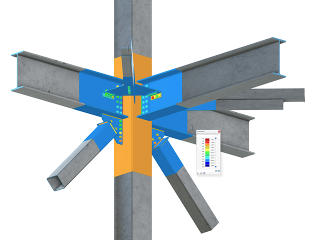
Complex Connection of Horizontal Beams to Column and Connection of Reinforcing Diagonals
The connection model was modeled using about 50 components. The model was created according to the real example of use in structure.
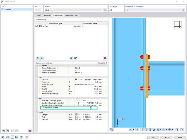
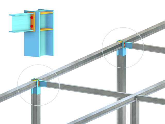
To determine the shear resistance of bolts, you can use the Steel Joints add-on to specify whether there is a shaft or a thread in the shear plane.
Go to Explanatory Video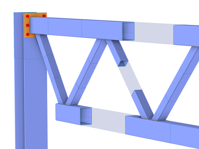
In the case of rectangular cross-sections, you can usually achieve a direct connection by using welds. However, you can also connect them to other cross-sections in the same way. Furthermore, other components such as end plates help you to connect the rectangular cross-sections to other structural components.

The building model is calculated in two phases:
- Global 3D calculation of the global model, where the slabs are modeled as a rigid plane (diaphragm) or as a bending plate
- Local 2D calculation of the individual floors
After the calculation, the results of the columns and walls from the 3D calculation and the results of the slabs from the 2D calculation are combined in a single model. This means that there is no need to switch between the 3D model and the individual 2D models of the slabs. The user only works with one model, saves valuable time, and avoids possible errors in the manual data exchange between the 3D model and the individual 2D ceiling models.
The vertical surfaces in the model can be divided into shear walls and opening lintels. The program automatically generates internal result members from these wall objects, so they can be designed as members according to any standard in the Concrete Design add-on.
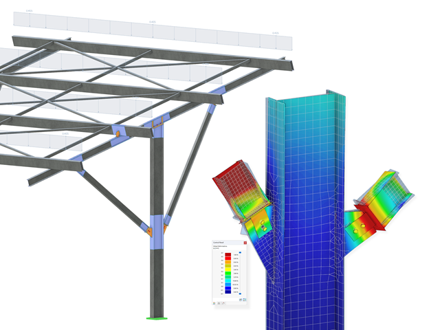
Steel bolted connections with gusset plates on the canopy structure.
Download the structural analysis model and open it with the finite element program RFEM 6 using Steel Joints Add-on.
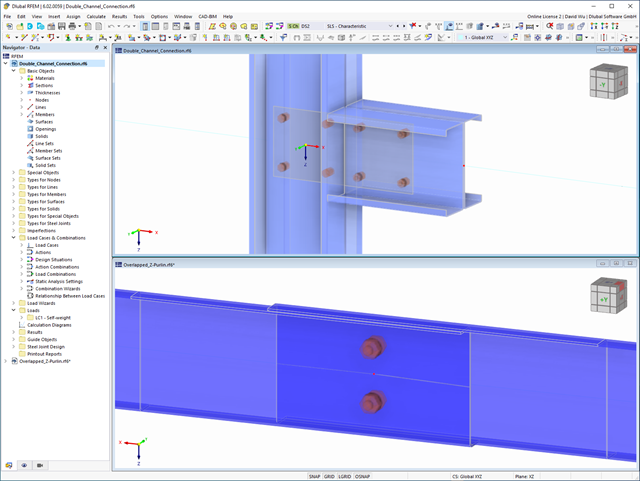
In the Steel Joint add-on, you can design the connections of members with composite cross-sections. Furthermore, you can perform joint design checks for almost all thin-walled cross-sections in the RFEM library.
Go to Explanatory Video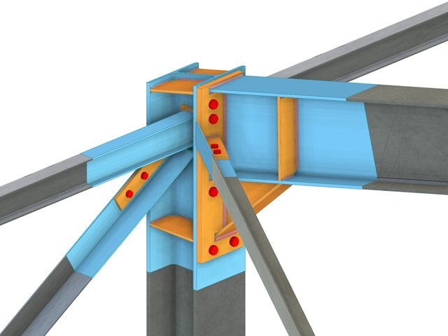
Design of a frame connection with taper and stiffened members. A stress analysis and a buckling stability analysis were carried out for the connection. To display the buckling results, the connection was converted into a separate model.
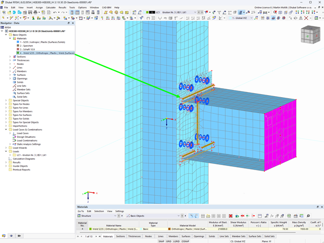
Here, the weld design becomes child's play. Using the specially developed material model "Orthotropic | Plastic | Weld (Surfaces)", you can calculate all stress components plastically. The stress τperpendicular is also considered plastically.
Using this material model you can design welds closer to reality and more efficiently.
Explanatory Video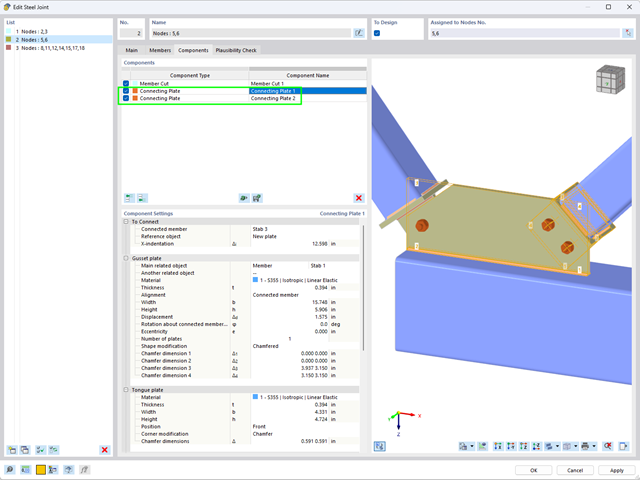
Using the "Connecting Plate" component, you can additionally and automatically create a new gusset plate in the Steel Joints add-on. This saves you separate components, and the other elements, such as a cap plate and a slide plate, are thus automatically taken into account with their dimensions.
Go to Explanatory VideoThe program supports you: Es ermittelt Schraubenkräfte anhand des FE-Analysemodells und wertet diese automatisch aus. Das Add-On führt die Nachweise der Schraubentragfähigkeit für Versagensfälle wie Zug, Abscheren, Lochleibung und Durchstanzen gemäß Norm durch und stellt alle benötigten Beiwerte übersichtlich dar.
Möchten Sie einen Schweißnahtnachweis führen? Die Schweißnähte werden als elastisch-plastische Flächenelemente modelliert, und deren Spannungen werden aus dem FE-Analysemodell ausgelesen. Die Plastizitätskriterien sind so eingestellt, dass sie Versagen gemäß AISC J2-4, J2-5 (Tragfähigkeit von Schweißnähten) und J2-2 (Festigkeit des Grundmetalls) darstellen. Der Nachweis kann mit den Teilsicherheitsbeiwerten des ausgewählten Nationalen Anhangs von EN 1993-1-8 erfolgen.
Der Nachweis der Bleche in der Verbindung wird plastisch durchgeführt, indem die vorhandene plastische Verzerrung mit der zulässigen plastischen Verzerrung verglichen wird. Die Standardeinstellung ist 5 % gemäß EN 1993-1-5, Anhang C, kann jedoch benutzerdefiniert angepasst werden, ebenso 5 % beim AISC 360.

Have you activated the Building Model add-on? Very good! This allows you to display the center of rigidity in tabular and graphical form. Use it for your dynamic analysis, for example.

As you've already learned, the results of a Modal Analysis load case are displayed in the program after a successful calculation. You can thus immediately see the first mode shape graphically or as an animation. You can also easily adjust the representation of the mode shape standardization. Do that directly in the Results navigator, where you have one of four options for the visualization of the mode shapes available for the selection:
- Scaling the value of the mode shape vector uj to 1 (considers the translation components only)
- Selecting the maximum translational component of the eigenvector and setting it to 1
- Considering the entire eigenvector (including the rotation components), selecting the maximum, and setting it to 1
- Setting the modal mass mi for each mode shape to 1 kg
You can find a detailed explanation of the mode shape standardization in the OnlineManual here.

- Numerous predefined components for easy input of typical connection situations (for example, end plates, angles, web plates)
- Universally applicable basic components (plates, welds, bolts, auxiliary planes) for the input of complex connection situations
- Graphical display of the connection geometry that is updated in parallel with the input
- The steel connection template included in the add-on allows you to select different connection types and apply them to your model
- The template provides connections from three categories: Rigid, Pinned, Truss
- Automatic adjustment of the connection geometry, even during subsequent editing of the structural components, due to the relative arrangement of the components to each other
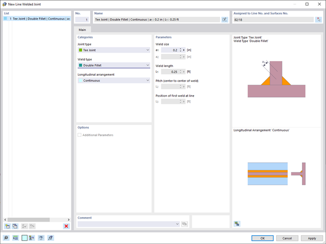
In RFEM 6, it is possible to define line welds between surfaces and to calculate the weld stresses using the Stress-Strain Analysis add-on.
The following joint types are available:
- Butt Joint
- Corner joint
- Lap Joint
- T-joint
Depending on the selected joint type, you can select the following weld types:
- Single Square
- Double Square
- Double Bevel
- Single V
- Double V
- Single U
- Double U
- Single J
- Double J

RFEM allows you to use a special line hinge to model the special properties of the connection between the reinforced concrete slab and masonry wall. This limits the transferable forces of the connection depending on the specified geometry. You guess right: This means that the material cannot be overloaded.
The program develops interaction diagrams that are applied automatically. They represent the various geometric situations and you can use them to determine the correct stiffness.

Compared to the RF‑/STEEL add-on module (RFEM 5 / RSTAB 8), the following new features have been added to the Stress-Strain Analysis add-on for RFEM 6 / RSTAB 9:
- Treatment of members, surfaces, solids, welds (line welded joints between two and three surfaces with subsequent stress design)
- Output of stresses, stress ratios, stress ranges, and strains
- Limit stress depending on the assigned material or a user-defined input
- Individual specification of the results to be calculated through freely assignable setting types
- Non-modal result details with prepared formula display and additional result display on the cross-section level of members
- Output of the design check formulas used

Is the calculation finished? The results of the modal analysis are then available both graphically and in tables. Display the result tables for the load case or the load cases of the modal analysis. Thus, you can see the eigenvalues, angular frequencies, natural frequencies, and natural periods of the structure at first glance. The effective modal masses, modal mass factors, and participation factors are also clearly displayed.
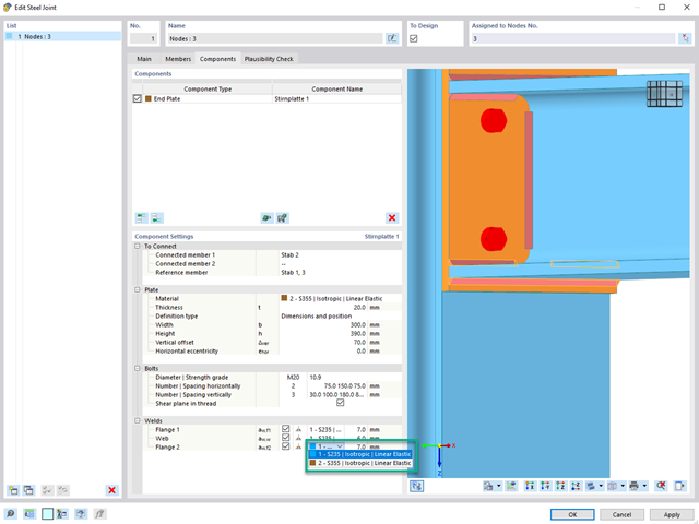
If a weld seam connects two plates with different materials, it is possible to select from a combo box in the Steel Joints add-on which one of both materials should be used for the weld seam.
Go to Explanatory Video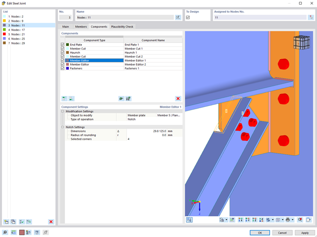
The "Member Editor" component allows you to modify the individual or several member plates in the Steel Joints add-on.
You can use the chamfer, notch, rounding, and hole operations with multiple shapes. It is possible to apply both operations, "Notch" and "Chamfer", for several member plates.
In this way, you can notch flanges from I-sections, for example (see the image).
Go to Explanatory Video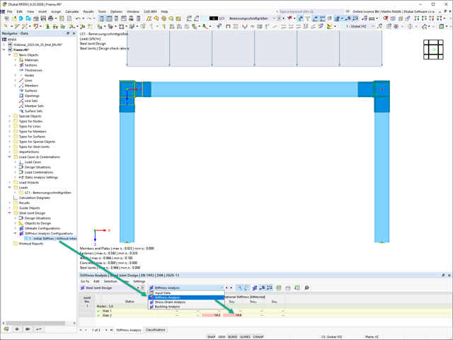
The initial stiffness Sj,ini is a decisive parameter for evaluating whether a connection can be characterized as rigid, non-rigid, or hinged.
In the “Steel Joints” add-on, you can calculate the initial stiffnesses Sj,ini according to Eurocode (EN 1993-1-8 Section 5.2.2) and AISC (AISC 360-16 Cl. E3.4) in relation to the internal forces N, My, and/or Mz.
The optional automatic transfer of initial stiffnesses allows for a direct transfer as member end hinge stiffnesses in RFEM. Then, the entire structure is recalculated and the resulting internal forces are automatically adopted as loads in the calculation and design of the connection models.
This automated iteration process eliminates the need for manual export and import of data, reducing the amount of work and minimizing potential sources of error.
Explanatory Video: Calculation of Initial Stiffness Sj,ini
After you have completed the design, the program takes care of clearly arranged results. Thus, the program shows you the resulting maximum stresses and stress ratios sorted by section, member/surface, solid, member set, x-location, and so on. In addition to the tabular result values, the add-on shows you the corresponding cross-section graphic with stress points, stress diagram, and values as well. You can relate the design ratio to any kind of stress type. The current location is highlighted in the RFEM/RSTAB model.
In addition to the tabular evaluation, the program offers you even more. You can also graphically check the stresses and design ratios on the RFEM/RSTAB model. It is possible for you to adjust the colors and values individually.
The display of result diagrams of a member or set of members enables you a targeted evaluation. For each design location, you can open the respective dialog box to check the design-relevant section properties and stress components of any stress point. Finally, you have the option of printing the corresponding graphic, including all design details.
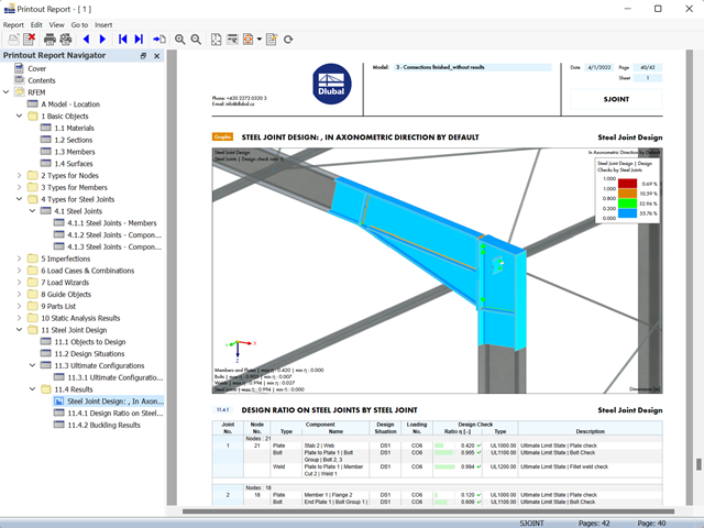
- The results of the connection design can be entered in the printout report
- When creating a new printout report, select the items added from the Steel Joints Add-on
- Use the tool 'Print Graphics to Printout Report' to insert graphics with the results of the connection, including the control panel, into the report
- Printout report contains the specifications of the connection components, design parameters, results and graphics
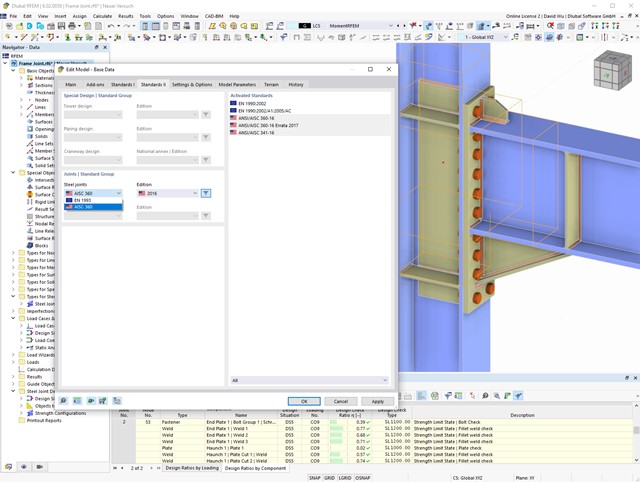
In the Steel Joints add-on, you can design connections according to the American standard ANSI/AISC 360‑16. The following design procedures are integrated:
- Load and Resistance Factor Design (LRFD)
- Allowable Stress Design (ASD)
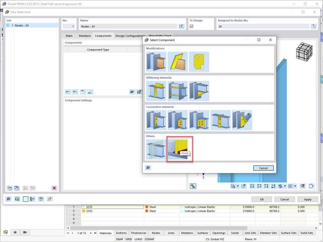
In addition to other predefined components in the design add-on for steel connections, the universal base component "General Weld" can be used to enter complex connection situations.

Is your goal to determine the number of mode shapes? The program offers you two methods for this. On the one hand, you can manually define the number of the smallest mode shapes to be calculated. In this case, the number of available mode shapes depends on the degrees of freedom (that is, the number of free mass points multiplied by the number of directions in which the masses act). However, it is limited to 9999. On the other hand, you can set the maximum natural frequency the way that the program determined the mode shapes automatically until reaching the natural frequency set.
.png?mw=640&hash=25998fe3470f8e1c154828f202ad6a728b30f00a)
Did you know that To calculate masonry structures, a nonlinear material model has been implemented in RFEM. It is based on the approach of Lourenco, a composite yield surface according to Rankine and Hill. This model allows you to describe and model the structural behavior of masonry and the different failure mechanisms.
The limit parameters were selected in such a way that the design curves used correspond to a normative design curve.
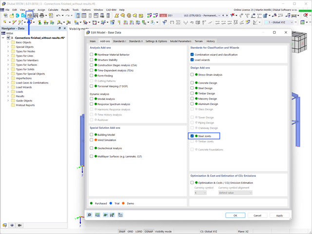
To design a Steel connection, you must have the Steel Joints Add-on enabled. The Add-ons in RFEM 6 are activated in the Add-ons tab of the Edit Model - Base Data window. If the Add-on is active, it is displayed in the navigator.
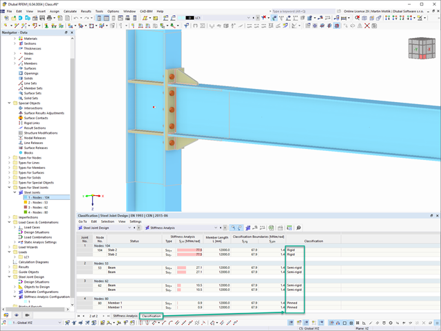
In the Steel Joints add-on, you can classify the joint stiffness.
In addition to the initial stiffness, the table also shows the limit values for hinged and rigid connections for the selected internal forces N, My, and/or Mz. The resulting classification is then displayed in tables as "hinged", "semi-rigid", or "rigid".
Go to Explanatory Video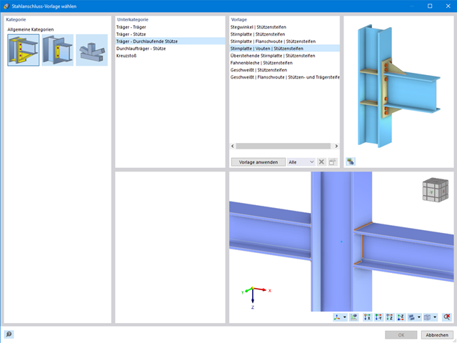
For joint components, you can check whether the stability failure is relevant. This requires the Structure Stability add-on for RFEM 6.
In this case, you calculate the critical load factor for all analyzed load combinations and the selected number of mode shapes for the connection model. Compare the smallest critical load factor with the limit value 15 from the standard EN 1993‑1‑1, Clause 5. Furthermore, you can make user-defined adjustment of the limit value. As a result of the stability analysis, the program displays the corresponding mode shapes graphically.
For the stability analysis, RFEM uses the adapted surface model to specifically recognize the local buckling shapes. You can also save and use the model of the stability analysis, including the results, as a separate model file.