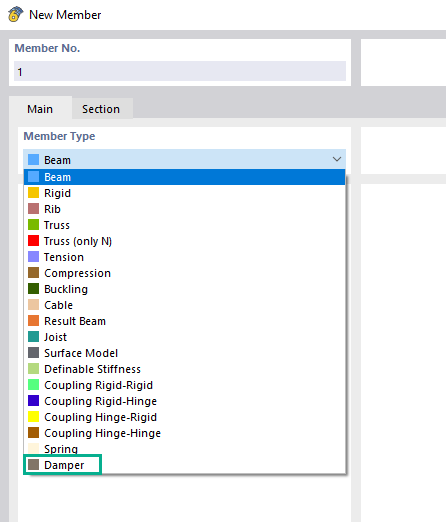
Using the "Damper" member type, you can define a damping coefficient, a spring constant, and a mass. This member type extends the possibilities within the Time History Analysis.
With regard to viscoelasticity, the "Damper" member type is similar to the Kelvin-Voigt model, which consists of the damping element and an elastic spring (both connected in parallel).
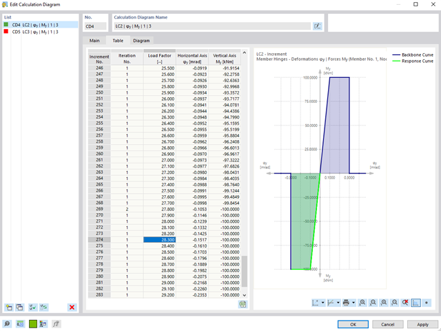
For calculation diagrams, the "2D | Hinge" is available. These hinge diagrams show the hinge response of load situations for nonlinear hinges.
For calculations with several load situations, such as is the case with pushover analyzes and time history analysis, you can evaluate the state of the hinge in each load step.
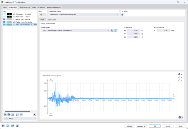
The Time History Analysis add-on provides you with accelerograms for the calculation. This extension allows for dynamic structural analysis of the acceleration-time diagrams.
There is an extensive library of earthquake records available for you, but you can also enter or import your own diagrams. The time history analysis is performed using the modal analysis or the linear implicit Newmark analysis.
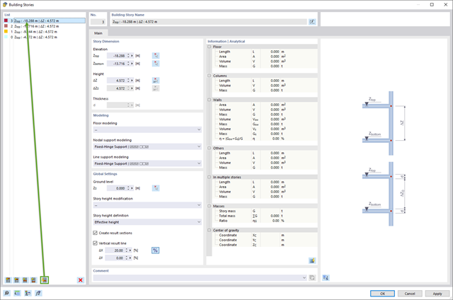
The building story generator in the Building Model add-on allows you to automatically create building stories, depending on the topology of the model.

For a response spectrum analysis of building models, you can display the sensitivity coefficients for the horizontal directions by story.
These key figures allow you to interpret the sensitivity to stability effects.
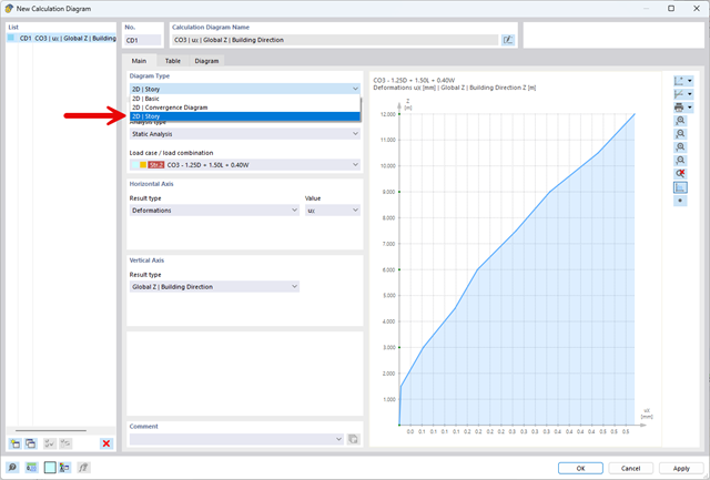
The "2D | Story" calculation diagram type is used to create result diagrams via the building axis. This allows you to easily analyze the behavior of the entire building under static and dynamic effects.
You can use this diagram type, for example, to visualize the seismic force over the building height.
- Analysis of time diagrams and accelerograms (acceleration-time diagrams exciting the supports of a structure)
- Combination of user-defined time diagrams with nodal, member, and surface loads, as well as free and generated loads
- Combination of several independent excitation functions
- Linear implicit Newmark analysis or modal analysis in time history
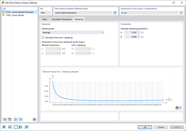
- Structural damping using Raleigh damping coefficients or Lehr's damping value
- Graphical display of results in calculation diagrams
- Result display in individual time steps or as an envelope during the entire time period
- Extensive library of seismic events (accelerograms)
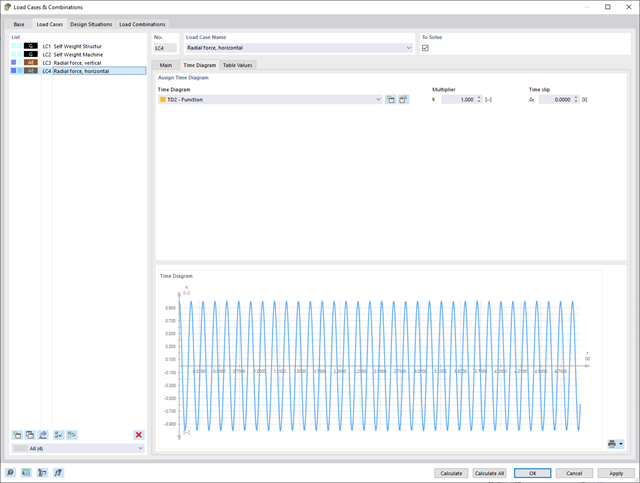
It is necessary to enter the required force-time diagrams. They can be combined in load cases or load combinations of the type Time History Analysis | Time Diagrams with the loading in order to define where and in which direction the force-time diagrams act.
The second option is to enter acceleration-time diagrams, which can be used in the load cases of the Time History Analysis | Accelerogram type.
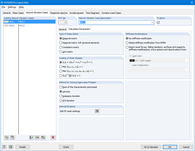
All calculation parameters are specified in the time history analysis settings. These include, for example, the type of analysis method and the maximum calculation time.
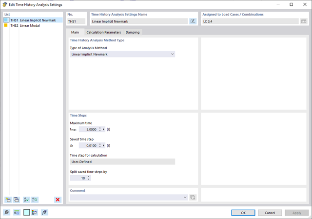
The time history analysis is performed with the modal analysis or the linear implicit Newmark analysis. The time history analysis in this add-on is limited to linear structural systems. Although the modal analysis represents a fast algorithm, it is necessary to use a certain number of eigenvalues to ensure the required accuracy of results.
The implicit Newmark analysis is a very precise method, independent of the number of eigenvalues used, but requires sufficient small time steps for the calculation.
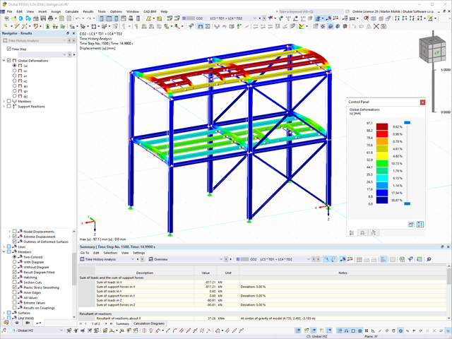
As soon as the program has completed the calculation, the summary of the results is listed. All result windows are integrated in the main program RFEM/RSTAB. You will find all the results arranged in tables; they can be displayed for each individual time step or as an envelope, and you also have the option of displaying the results graphically as well as animating them.
The results from the time history analysis can be displayed in the calculation diagrams. All the results are shown as a function of time. You can export the numeric values to MS Excel.
All result tables and graphics are part of the RFEM/RSTAB printout report. In this way, you can ensure clearly arranged documentation. You can also export the tables to MS Excel.

Using the "Load Transfer Only" story type, you can consider slabs without stiffness effect in and out of the plane in the Building Model add-on. This element type collects the loads on the slab and transfers them to the supporting elements of a 3D model. Thus, you can simulate secondary components, such as grillage and similar load distribution elements, without any further effect in the 3D model.
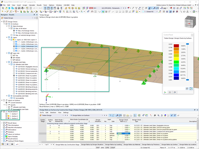
You can graphically evaluate result sections for the timber surface design. This can be done in the RFEM graphic as well as in the result history window. The sections can be placed at any location in order to evaluate the design results in detail.
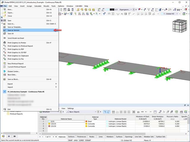
It is possible to save different model versions within a model by using the Save as Version function. In the Base Data of the model, the different model versions can be displayed in the History tab.

Are you afraid that your project will end in the digital tower of Babel? The Building Model add-on for RFEM supports you in your work on a construction project with several stories. It allows you to define a building by means of stories at specified elevations. You can adjust the stories in many ways afterwards and also select the story slab stiffness. Information about the stories and the entire model (center of gravity, center of rigidity) is displayed for you in tables and graphics.
More About Building Model
- Consideration and display of story masses
- Listing of structural elements and their information
- Automated creation of result sections on shear walls
- Output of section resultants in global direction for determining shear forces
- Optional definition of rigid diaphragm by story (story modeling)
- Stiffness type Floor Slab - Rigid Diaphragm
- Defining floor sets,
- for example, calculation of slabs as a 2D position within the 3D model
- Shear walls: Automatic definition of result members with any cross-section
- Design of rectangular cross-sections using the Concrete Design add-on
- Definition of deep beams, design possible using the Concrete Design add-on
- Tabular output of story actions, interstory drift, and center points of mass and stiffness, as well as the forces in shear walls
- Separate result display of the floor and stiffening design
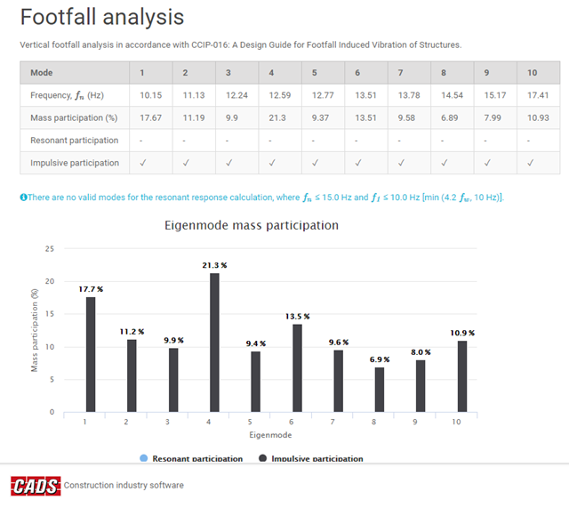
- Overall maximum response factors and critical nodes
- Resonant analysis (maximum response factor, RMS acceleration, critical node, critical frequency)
- Impulsive (transient) analysis (maximum response factor, peak acceleration/velocity, RMS acceleration/velocity, critical node, critical frequency)
- Vibration dose values for both resonant and impulsive analyses
Charts
- Response factor vs walking frequency
- Mass participation vs eigenmodes
- Velocity time history
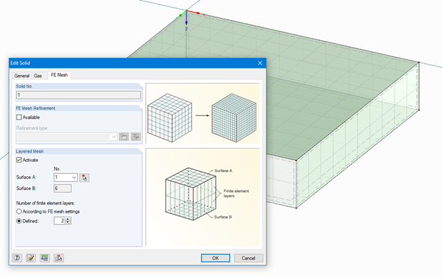
The stiffness of gas given by the ideal gas law pV = nRT can be considered in the nonlinear dynamic analysis.
The calculation of gas is available for accelerograms and time diagrams for both the explicit analysis and the nonlinear implicit Newmark analysis. To determine the gas behavior correctly, at least two FE layers for gas solids should be defined.
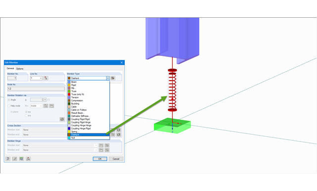
The member type 'Dashpot' can be used for time history analyzes in RFEM/RSTAB with the add-on modules RF-/DYNAM Pro - Forced Vibrations and RF-/DYNAM Pro - Nonlinear Time History. This linear viscous damping element considers forces dependent on velocity.
With regard to viscoelasticity, the member type 'Dashpot' is similar to the Kelvin-Voigt model, which consists of the damping element and an elastic spring (both connected in parallel).
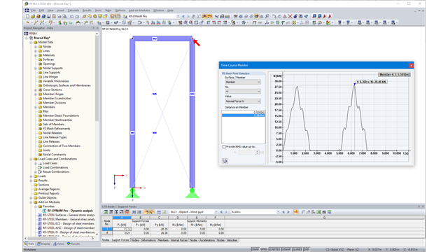
Due to the integration of RF‑/DYNAM Pro in RFEM or RSTAB, you can incorporate numeric and graphic results from RF‑/DYNAM Pro - Nonlinear Time History to the global printout report. Also, all RFEM and RSTAB options are available for a graphical visualization. The results of the time history analysis are displayed in a time history diagram.
The results are displayed as a function of time and the numerical values can be exported to MS Excel. Result combinations can be exported, either as a result of a single time step or the most unfavorable results of all time steps are filtered out.
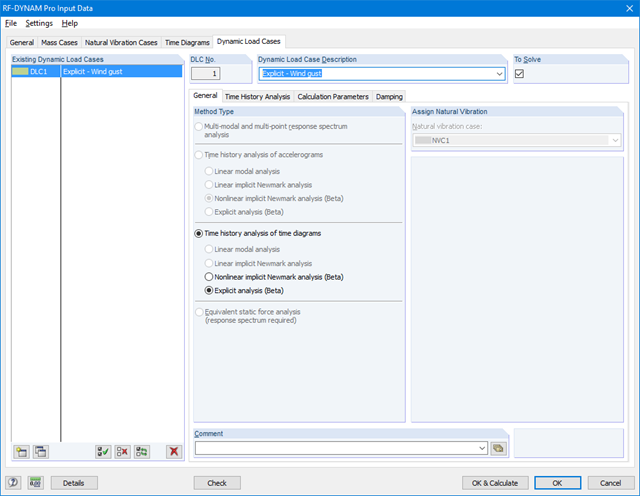
Calculation in RFEM
The nonlinear time history analysis is performed with the implicit Newmark analysis or the explicit analysis. Both are direct time integration methods. The implicit analysis requires small time steps to provide precise results. The explicit analysis determines the required time step automatically to provide the stability to the solution. The explicit analysis is suitable for the analysis of short excitations, such as impulse excitation, or an explosion.
Calculation in RSTAB
The nonlinear time history analysis is performed with the explicit analysis. This is a direct time integration method and determines the required time step automatically in order to provide the solution stability.

RF-/DYNAM Pro - Nonlinear Time History is integrated in the structure of RF‑/DYNAM Pro - Forced Vibrations and extended by two nonlinear analysis methods (one nonlinear analysis in RSTAB).
Force-time diagrams can be entered as transient, periodic, or as a function of time. Dynamic load cases combine the time diagrams with the static load cases, which provides high flexibility. Furthermore, it is possible to define time steps for the calculation, structural damping, and export options in the dynamic load cases.

- Nonlinear member types, such as tension and compression members or cables
- Member nonlinearities, such as failure, tearing, yielding under tension or compression
- Support nonlinearities, such as failure, friction, diagram, and partial activity
- Release nonlinearities, such as friction, partial activity, diagram, and fixed if positive or negative internal forces
.png?mw=640&hash=8cfd0c4bd093c03de543d147ffbf6f5c9250634a)
- User-defined time diagrams as a function of time, in tabular form, or as harmonic loads
- Combination of the time diagrams with RFEM/RSTAB load cases or combinations (enables definition of nodal, member, and surface loads, as well as free and generated loads varying over time)
- Combination of several independent excitation functions
- Nonlinear time history analysis with the implicit Newmark analysis (RFEM only) or the explicit analysis
- Structural damping using Rayleigh damping coefficients or Lehr's damping
- Direct import of initial deformations from a load case or combination (RFEM only)
- Stiffness modifications as initial conditions; for example, axial force effect, deactivated members (RSTAB only)
- Graphical display of results in a time history diagram
- Export of results in user-defined time steps or as an envelope
Due to the integration of RF‑/DYNAM Pro in RFEM / RSTAB, you can incorporate numeric and graphic results from RF‑/DYNAM Pro – Forced Vibrations in the global printout report. Also, all RFEM options are available for a graphical visualization.
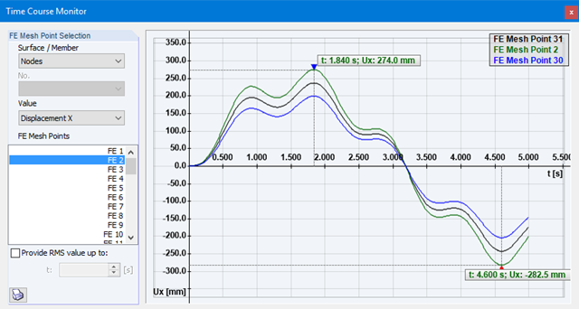
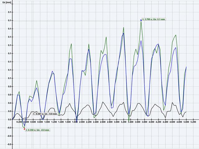
The results of the time history analysis are displayed in a time course monitor. All results are displayed as a function of time. You can export the numeric values to MS Excel.
In the case of a time history analysis, you can export results of the individual time steps or filter most unfavourable results of all time steps.
The response spectrum analysis generates result combinations. Internally, the modal contributions and the directional components of earthquake actions are combined.
The time history analysis is performed with the modal analysis or the linear implicit Newmark analysis. The time history analysis in this add‑on module is restricted to linear systems. Although the modal analysis represents a fast algorithm, it is necessary to use a certain number of eigenvalues to ensure the required accuracy of results.
The implicit Newmark analysis is a very precise method, independent of the number of eigenvalues used, but requires sufficient small time steps for calculation. For the response spectra analysis, equivalent static loads are calculated internally. A linear static analysis is performed subsequently.
It is necessary to enter the required response spectra, accelerations, or time diagrams. Dynamic load cases define the location and direction of response spectra effects as well as acceleration time, or force-time excitations.
Timing diagrams are combined with static load cases, which provides great flexibility. For the time history analysis, you can import the initial deformation from any load case or load combination.
- Combination of user-defined time diagrams with load cases or load combinations (nodal, member, and surface loads, as well as free and generated loads, can be combined with time-variable functions)
- Combination of several independent excitation functions
- Extensive library of seismic events (accelerograms)
- Linear implicit Newmark analysis or modal analysis in time history
- Structural damping using Rayleigh damping coefficients or Lehr's damping
- Direct import of initial deformations from a load case or combination
- Graphical display of results in a time history diagram
- Export of results in user-defined time steps or as an envelope
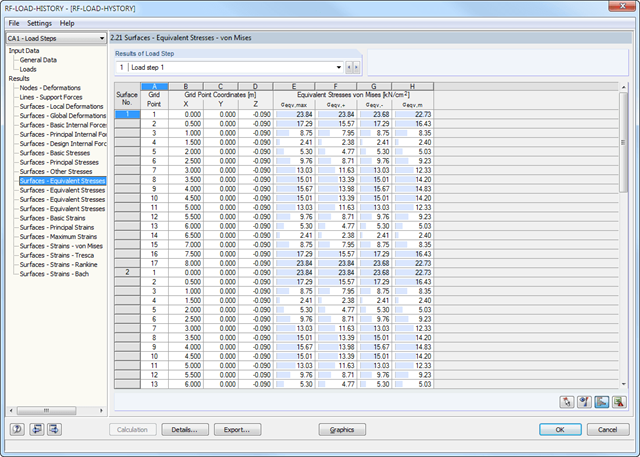
After the calculation, you can evaluate the results of the individual load steps directly in the module windows or graphically in a structural model.
The results include, for example, deformations, stresses, and internal forces of surfaces, as well as deformations and stresses of solids. It is possible to export the result combinations for each load step to RFEM. You can use these enveloping combinations for further designs in the other RFEM add-on modules.
All input data and results of the add-on module are part of the global RFEM printout report.
The calculation is performed successively for each load step. Permanent (plastic) deformations of previous load steps are considered when calculating further load steps. This way, it is also possible to perform a calculation with a structure relief.
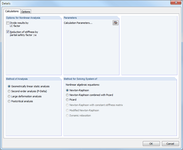
The loads of the individual steps are added up (depending on the signs) throughout the calculation process. You can freely select the method of analysis (linear static, second-order, large deformation, and postcritical analysis). Furthermore, the module manages the global calculation settings.
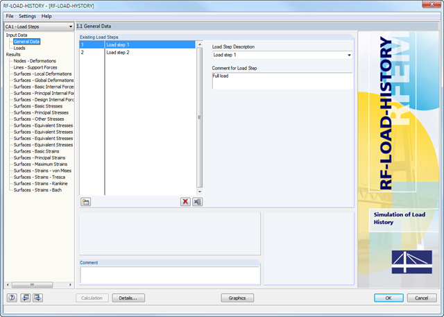
After defining the entire model and loading in RFEM, it is possible to enter load steps and descriptions in the 1.1 General Data window.
In Window 1.2 Loads, you can assign the load cases or load combinations to the different load increments. It is possible to multiply them by a load factor.