Program RFEM 6 do analizy statyczno-wytrzymałościowej jest podstawą systemu modułowego. Program główny RFEM 6 służy do definiowania konstrukcji, materiałów i obciążeń płaskich i przestrzennych układów konstrukcyjnych składających się z płyt, ścian, powłok i prętów. Program umożliwia również tworzenie konstrukcji mieszanych oraz modelowanie elementów bryłowych i kontaktowych.
RSTAB 9 to wydajne oprogramowanie do obliczeń konstrukcji szkieletowych 3D, odzwierciedlające aktualny stan wiedzy i pomagające inżynierom sprostać wymaganiom współczesnej inżynierii lądowej.
Często zbyt długo zajmujesz się obliczaniem przekrojów? Oprogramowanie firmy Dlubal i program samodzielny RSECTION ułatwiają pracę, określając i przeprowadzając analizę naprężeń dla różnych przekrojów.
Czy zawsze wiesz, skąd wieje wiatr? Oczywiście od strony innowacji! RWIND 3 to program, który wykorzystuje cyfrowy tunel aerodynamiczny do numerycznej symulacji przepływu wiatru. Program symuluje przepływ wokół dowolnej geometrii budynku i określa obciążenia wiatrem na powierzchnie.
Szukasz narzędzia do przeglądu stref obciążenia śniegiem, wiatrem i trzęsieniem ziemi? Dobrze trafiłeś! Skorzystaj z narzędzia do geolokalizacji do szybkiego i skutecznego definiowania obciążenia śniegiem, prędkości wiatru, obciążenia trzęsieniem ziemi, zgodnie z Eurokodem i innymi międzynarodowymi normami.
Chcesz wypróbować możliwości programów Dlubal Software? To Twoja szansa! Dzięki 90-dniowej pełnej wersji, możesz w pełni przetestować wszystkie nasze programy.
Dostępne są dwie opcje: eine automatische Zeitschrittwahl und eine manuelle. Gerade für eine Struktur mit Nichtlinearitäten wird immer empfohlen, den Zeitschritt manuell zu wählen, da die automatische Ermittlung nur anhand der definierten Akzelerogramme bzw. Zeitdiagramme durchgeführt wird. Dafür sollte eine Zeitschrittkonvergenzstudie durchgeführt werden, welche die Berechnungszeit und die Genauigkeit ins Verhältnis setzt.
Der zu wählende Zeitschritt ist von vielen Faktoren abhängig, darunter die Erregungsfrequenz, die Frequenz und die Größe der Struktur, sowie der Grad an Nichtlinearitäten. Es kann also keine allgemeingültige Aussage über die Größe des Zeitschritts getroffen werden.
Um eine ausreichende Genauigkeit zu erreichen, sollte die maßgebende Periode T = 1/f in etwa 20 Schritte unterteilt werden, d. h. der Zeitschritt Δt ist wie folgt zu wählen:
$\mathrm{Δt}\;<\frac{\mathrm T}{20}\;=\;\frac1{20\mathrm f}\;=\;\frac{\mathrm\pi}{10\mathrm\omega\;}$
Für transient definierte Anregungen, wie Akzelerogramme oder tabellierte Zeitdiagramme, sollte der kürzeste Zeitabschnitt in 7 Schritte unterteilt werden:
$\mathrm{Δt}\;=\;\frac{\mathrm{Min}\left\{{\mathrm t}_{\mathrm i+1}\right.-\;{\mathrm t}_{\mathrm i}\}\;}7$
Unabhängig der Berechnung werden Zeitschritte zum Speichern der Ergebnisse angegeben.