39 Wyniki
Wyświetl wyniki:
Sortuj według:

- 002876
- Ogólne informacje
- Projektowanie konstrukcji betonowych RFEM 6
- Projektowanie konstrukcji betonowych RSTAB 9
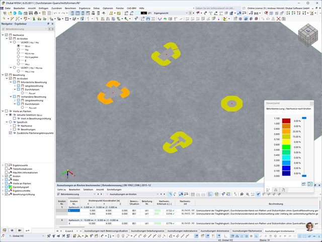
W przypadku obliczeń betonu wyniki zbrojenia można wyświetlić w tabelach osobno w zależności od sytuacji obliczeniowych.

- 002161
- Ogólne informacje
- Optymalizacja i koszty | Szacowanie emisji CO2 RFEM 6
- Optymalizacja i koszty | Szacowanie emisji CO2 RSTAB 9
Obie metody optymalizacji mają jedną wspólną cechę. Na końcu procesu wyświetlają listę wariacji modelu na podstawie przechowywanych danych. Można tu znaleźć szczegóły na temat wyniku decydującego dla optymalizacji i odpowiadające mu wartości parametrów. Lista jest zorganizowana w porządku malejącym. Zakładane najlepsze rozwiązanie znajduje się na górze. W takim przypadku wynik optymalizacji wraz z wyznaczoną wartością jest najbardziej zbliżony do kryterium optymalizacji. Wszystkie dodatkowe wyniki pokazują wykorzystanie < 1. Ponadto, po zakończeniu analizy, program dostosuje wartości na globalnej liście parametrów, aby odpowiadały tym dla optymalnego rozwiązania.
W oknach dialogowych materiałów znajdują się dodatkowe zakładki "Oszacowanie kosztów" i "Oszacowanie emisji CO2". Tutaj wyświetlane są indywidualne szacunkowe sumy przydzielonych prętów, powierzchni i objętości na jednostkę masy, objętości i powierzchni. Dodatkowo zakładki te podają całkowity koszt i emisję wszystkich przydzielonych do konstrukcji materiałów. Zapewnia to dobry przegląd projektu.

W rozszerzeniu Projektowanie konstrukcji betonowych dla programu RFEM 6 można przeprowadzić obliczenia odporności ogniowej ścian i płyt żelbetowych zgodnie z uproszczoną metodą tabelaryczną (EN 1992-1-2, rozdział 5.4.2 oraz tabele 5.8 i 5.9).
- 002801
- Ogólne informacje
- Projektowanie konstrukcji betonowych RFEM 6
- Projektowanie konstrukcji betonowych RSTAB 9
Masz indywidualne przekroje słupów i ścian o różnej geometrii, które wymagają obliczenia nośności na przebicie?
Nie ma problemu. W programie RFEM 6 można przeprowadzić obliczenia na przebicie nie tylko dla przekrojów prostokątnych i okrągłych, ale także dla dowolnego kształtu przekroju.

- 002109
- Ogólne informacje
- Optymalizacja i koszty | Szacowanie emisji CO2 RFEM 6
- Optymalizacja i koszty | Szacowanie emisji CO2 RSTAB 9
Masz pytania dotyczące programu? Optymalizacja konstrukcji w programach RFEM i RSTAB jest uzupełnieniem parametrycznego wprowadzania danych. Jest to proces równoległy, niezależny od rzeczywistych obliczeń modelu wraz ze wszystkimi jego zwykłymi definicjami obliczeń i obliczeń. Rozszerzenie zakłada, że model lub blok jest zbudowany w kontekście parametrycznym i jest kontrolowany przez globalne parametry kontrolne typu "optymalizacja". Dlatego te parametry kontrolne mają dolną i górną granicę oraz wielkość kroku w celu ograniczenia zakresu optymalizacji. Aby znaleźć optymalne wartości parametrów kontrolnych, należy określić kryterium optymalizacji (na przykład minimalny ciężar) przy wyborze metody optymalizacji (na przykład optymalizacja roju cząstek).
Oszacowanie kosztów i emisji CO2 można znaleźć już w definicjach materiałów. Obie opcje można aktywować osobno w każdej definicji materiału. Oszacowanie oparte jest na koszcie jednostkowym lub jednostkowej wartości emisji dla prętów, powierzchni oraz brył. W tym przypadku można wybrać, czy jednostki mają zostać podane według masy, objętości czy powierzchni.

- 002108
- Ogólne informacje
- Optymalizacja i koszty | Szacowanie emisji CO2 RFEM 6
- Optymalizacja i koszty | Szacowanie emisji CO2 RSTAB 9
- Technologia sztucznej inteligencji (AI): Optymalizacja roju cząstek (PSO)
- Optymalizacja konstrukcji ze względu na minimalny ciężar lub deformację
- Możliwość zastosowania dowolnej liczby parametrów optymalizacyjnych
- Określanie zakresów zmiennych
- Optymalizacja przekrojów i materiałów
- Typy definicji parametrów
- Optymalizacja | Rosnąco, czyli optymalizacja | Malejąca
- Zastosowanie parametrycznych modeli i bloków
- Parametryzacja bloków w języku JavaScript na podstawie kodu
- Optymalizacja z uwzględnieniem wyników obliczeń
- Tabelaryczne przedstawienie najlepszych mutacji modelu
- Wyświetlanie w czasie rzeczywistym mutacji modelu w procesie optymalizacji
- Kalkulacja kosztów modelu dzięki zadanym cenom jednostkowym
- Określanie potencjału tworzenia efektu cieplarnianego (GWP-global warming potential) na etapie tworzenia modelu poprzez szacowanie równoważnej emisji CO2
- Określanie jednostkowych wskaźników zależnych od masy, objętości i powierzchni (cena i emisja CO2)

- 002110
- Ogólne informacje
- Optymalizacja i koszty | Szacowanie emisji CO2 RFEM 6
- Optymalizacja i koszty | Szacowanie emisji CO2 RSTAB 9
Istnieją dwie metody optymalizacji, dzięki którym można znaleźć optymalne wartości parametrów według kryterium ciężaru lub odkształcenia.
Najbardziej wydajną metodą o najkrótszym czasie obliczeń jest optymalizacja roju cząstek zbliżona do naturalnej (PSO). Czy słyszałeś lub czytałeś o tym? Ta technologia sztucznej inteligencji (AI) ma silną analogię do zachowania stad zwierząt szukających miejsca odpoczynku. W takich rojach można znaleźć wiele osób (por. rozwiązanie optymalizacyjne - na przykład waga), które lubią przebywać w grupie i podążać za ruchem grupy. Załóżmy, że każdy pręt roju musi zostać poddany spoczynkowi w optymalnym miejscu (por. najlepsze rozwiązanie - na przykład najniższa waga). Potrzeba ta wzrasta wraz ze zbliżaniem się do miejsca odpoczynku. Na zachowanie roju mają zatem wpływ również właściwości przestrzeni (por. wykres wyników).
Dlaczego wycieczka do biologii? Po prostu - proces PSO w RFEM lub RSTAB przebiega w podobny sposób. Proces obliczeń rozpoczyna się od wyniku optymalizacji poprzez losowe przypisanie parametrów, które mają zostać zoptymalizowane. Wielokrotnie określa nowe wyniki optymalizacji ze zróżnicowanymi wartościami parametrów, które opierają się na doświadczeniach z wcześniej przeprowadzonych mutacji modelu. Proces jest kontynuowany do momentu osiągnięcia określonej liczby możliwych mutacji modelu.
Jako alternatywa dla tej metody program oferuje również metodę przetwarzania wsadowego. Metoda ta ma na celu sprawdzenie wszystkich możliwych mutacji modelu poprzez losowe określanie wartości parametrów optymalizacji, aż do osiągnięcia określonej liczby możliwych mutacji modelu.
Po obliczeniu mutacji modelu obydwa warianty sprawdzają również odpowiednie aktywowane wyniki obliczeń rozszerzeń. Ponadto zapisuje on wariant z odpowiednim wynikiem optymalizacji i przypisaniem wartości parametrów optymalizacji, jeżeli wykorzystanie jest < 1.
Na podstawie odpowiednich sum poszczególnych materiałów można określić szacunkowe koszty całkowite i emisję. Na sumę materiałów składają się zależne od ciężaru, objętości i powierzchnie elementów prętowych, powierzchniowych i bryłowych.

W rozszerzeniu Projektowanie konstrukcji betonowych można zdefiniować istniejące pionowe zbrojenie na ścinanie. Jest to następnie uwzględniane przy obliczaniu wytrzymałości na przebicie.
- 002720
- Ogólne informacje
- Analiza stateczności konstrukcji RFEM 6
- Analiza stateczności konstrukcji RSTAB 9
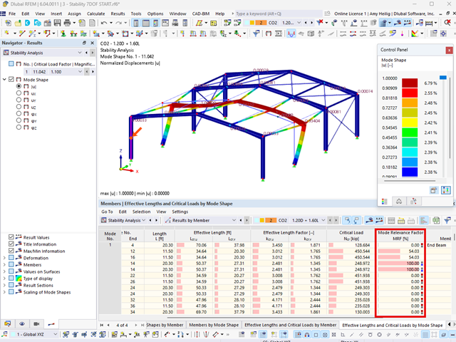
Stosując modalny współczynnik istotności (MRF) można ocenić, w jakim stopniu poszczególne elementy konstrukcyjne przyczyniają się do powstania rzeczywistego kształtu wyboczenia. Obliczenia opierają się na energii względnego odkształcenia sprężystego każdego pojedynczego pręta.
Dzięki MRF można rozróżnić lokalne i globalne kształty wyboczenia. Jeżeli kilka prętów ma znaczny MRF (np. > 20%), bardzo prawdopodobna jest niestateczność całej konstrukcji lub jej części. Jeżeli jednak suma wszystkich MRF dla kształtu drgań wynosi około 100%, należy spodziewać się lokalnego problemu ze statecznością (np. wyboczenia pojedynczego pręta).
Ponadto MRF może być wykorzystany do określenia obciążeń krytycznych i równoważnych długości wyboczeniowych poszczególnych prętów (np. do analizy stateczności). Kształty wyboczenia, dla których dany pręt ma małe wartości MRF (np. <20%), mogą zostać w tym kontekście pominięte.
MRF jest wyświetlany według kształtów wyboczenia w tabeli wyników w sekcji Analiza stateczności --> Wyniki według prętów --> Długości efektywne i obciążenia krytyczne.
- 002073
- Ogólne informacje
- Analiza stateczności konstrukcji RFEM 6
- Analiza stateczności konstrukcji RSTAB 9
- Obliczanie modeli składających się z elementów prętowych, powłokowych i bryłowych
- Nieliniowa analiza stateczności
- Możliwość uwzględniania sił osiowych od wstępnego sprężenia
- Cztery dostępne solvery do rozwiązywania równań dla efektywnego obliczania różnych modeli konstrukcyjnych
- Opcjonalne uwzględnianie zmian w sztywności w programie RFEM/RSTAB
- Wyszukiwanie postaci wyboczeniowych o krytycznym mnożniku obciążenia większym niż zadany przez użytkownika (metoda "przesunięcia")
- Możliwość określania wektorów własnych dla modeli niestatecznych (w celu zidentyfikowania przyczyny niestateczności)
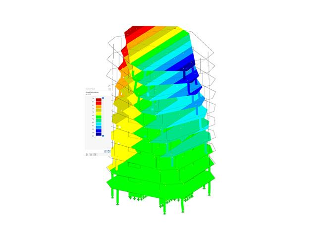
- Wizualizacja postaci niestateczności
- Podstawa określania imperfekcji