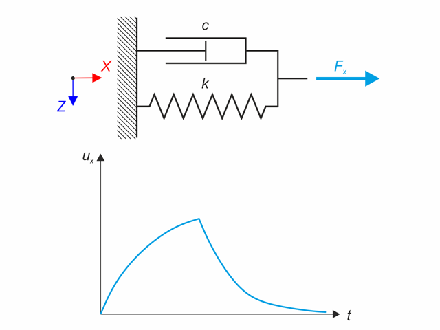
Kelvin-Voigt material model consists of the linear spring and viscous damper connected in parallel. In this verification example there is tested the time behaviour of this model during the loading and relaxation in a time interval 24 hours. The constant force Fx is applied for 12 hours and the rest 12 hours is the material model free of load (relaxation). The deformation after 12 and 20 hours is evaluated. Time History Analysis with Linear Implicit Newmark method is used.
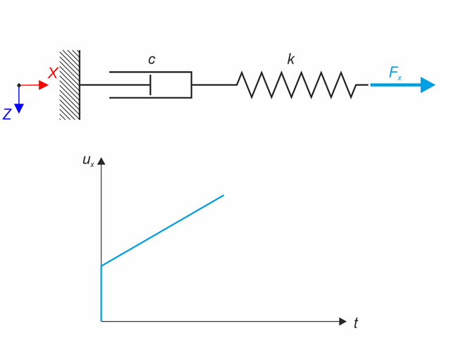
Maxwell material model consists of the linear spring and viscous damper connected in series. In this verification example there is tested the time behaviour of this model. The Maxwell material model is loaded by constant force Fx. This force causes initial deformation thanks to the spring, the deformation is then growing in time due to the damper. The deformation is observed at time of loading (20 s) and at the end of the analysis (120 s). Time History Analysis with Linear Implicit Newmark method is used.
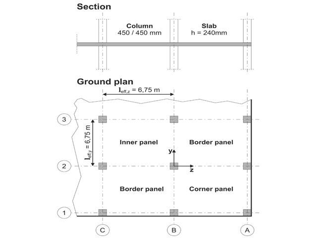
The model is based on the example 4 of [1]: Point-supported slab.
The flat slab of an office building with crack-sensitive lightweight walls is to be designed. Inner, border and corner panels are to be investigated. The columns and the flat slab are monolithically joined. The edge and corner columns are placed flush with the edge of the slab. The axes of the columns form a square grid. It is a rigid system (building stiffened with shear walls).
The office building has 5 floors with a floor height of 3.000 m. The environmental conditions to be assumed are defined as "closed interior spaces". There are predominantly static actions.
The focus of this example is to determine the slab moments and the required reinforcement above the columns under full load.
The model is based on the example 4 of [1]: Point-supported slab. The internal forces and the required longitudinal reinforcement can be found the in verification example 1022. In this example, punching is examined in the axis B/2.
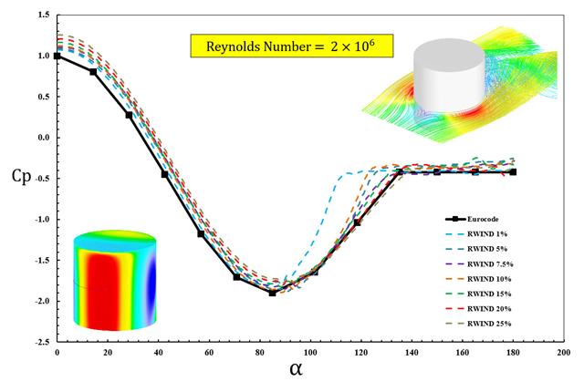
Das Architectural Institute of Japan (AIJ) hat eine Reihe an bekannten Benchmark-Szenarien für Windsimulation vorgestellt.
Der Nachfolgende Beitrag dreht sich dabei um den "Case A - high-rise building with a 2:1:1 shape".
Im Folgenden wird das beschriebene Szenario in RWIND2 nachgebildet und die Ergebnisse mit den simulierten und der experimentellen Resultate des AIJ verglichen.
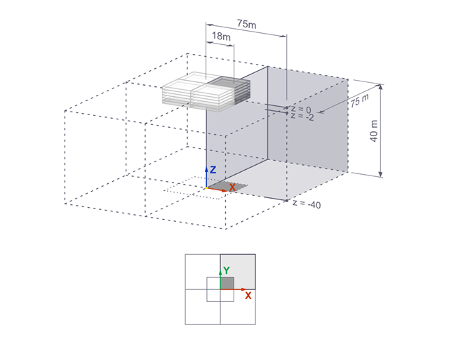
The settlements of a rigid square foundation on a lacustrine clay [1] are calculated with RFEM. One quarter of the foundation is modelled. The foundation has a width of 75.0 m in both sides. Construction stages are used to generate the results.
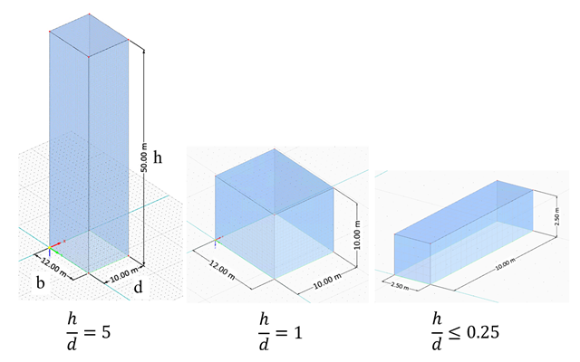
In the current validation example, we investigate wind force coefficient (Cf) of cube shapes with EN 1991-1-4 [1]. There are three dimensional cases that we will explain more about if in the next part.
The available standards, such as EN 1991-1-4 [1], ASCE/SEI 7-16, and NBC 2015 presented wind load parameters such as wind pressure coefficient (Cp) for basic shapes. The important point is how to calculate wind load parameters faster and more accurately rather than working on time-consuming as well as sometimes complicated formulas in standards.

An ASTM A992 W-shaped member is selected to carry a dead load of 30.000 kips and a live load of 90.000 kips in tension. Verify the member strength using both LRFD and ASD.
An ASTM A992 14×132 W-shaped column is loaded with the given axial compression forces. The column is pinned top and bottom in both axes. Determine whether the column is adequate to support the loading shown in Figure 1 based on LRFD and ASD.
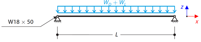
Consider an ASTM A992 W 18x50 beam forspan and uniform dead and live loads as shown in Figure 1. The member is limited to a maximum nominal depth of 18 inches. The live load deflection is limited to L/360. The beam is simply supported and continuously braced. Verify the available flexural strength of the selected beam, based on LRFD and ASD.

An ASTM A992 W 24×62 beam with end shears of 48.000 and 145.000 kips from the dead and live loads, respectively, is shown in Figure 1. Verify the available shear strength of the selected beam, based on LRFD and ASD.
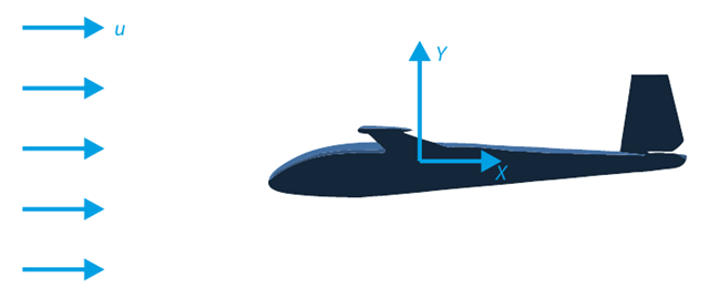
The goal of this verification example is to analyze the fluid flow around the glider. The task is to determine the drag coefficient and the lift coefficient with respect to the angle of attack. These coefficients can also be drawn into the graph of the drag polar. The limit angle for laminar fluid flow around the wing profile can also be determined from the velocity field. The available 3D CAD model (STL file) is used in RWIND 2.
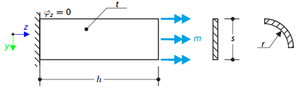
A thin plate is fixed on one side and loaded by means of distributed torque on the other side. First, the plate is modeled as a planar plate. Furthermore, the plate is modeled as one-fourth of the cylinder surface. The width of the planar model is equal to the length of one-fourth of the circumference of the curved model. The curved model thus has almost equal torsional constant to the planar model.
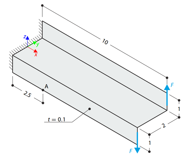
A Z-Section Cantilever is fully fixed at the end and loaded by a torque which, in the case of a shell model, is represented by a couple of shear forces. Determine the axial stress at point A (at mid-surface). The problem is defined according to The Standard NAFEMS Benchmarks.
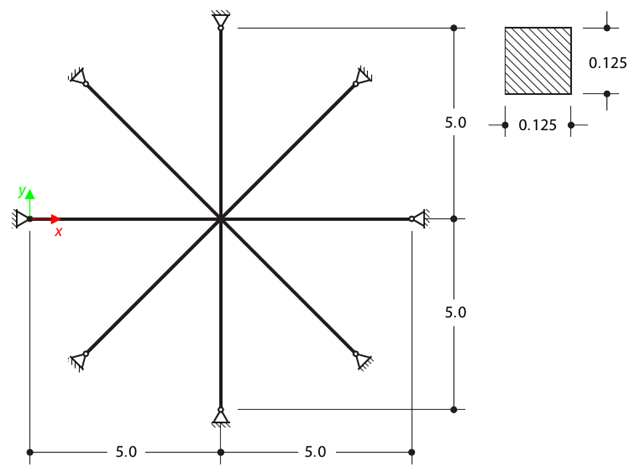
Determine the first sixteen natural frequencies of a double cross with a square cross-section. Each of the eight arms is modeled by means of four beam elements and has a pin support at the end (the x- and y-deflections are restricted). The vibrations are considered only in plane xy. The problem is defined according to The Standard NAFEMS Benchmarks.
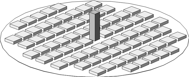
The verification example describes wind loads in several wind directions on a model of a group of buildings. The model consists of eight cubes. The velocity fields obtained by the RWIND simulation are compared with the measured values from the experiment. The experimental data are measured using a thermistor anemometer in the wind tunnel.
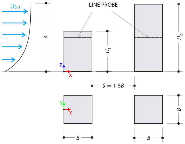
The verification example describes pressure loads on the walls of buildings in tandem arrangement located at ground level. The buildings are simplified to rectangular objects and scaled down while maintaining the elevation ratios. The pressure distribution on the walls of the model of a medium-high building was conducted by an experiment. The chosen results (pressure coefficient Cp) are compared with the measured values.
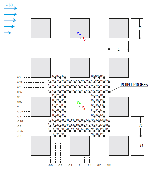
The verification example describes the steady-state flow around a high-rise building in city blocks (scaled model). The example is given by the Architectural Institute of Japan (AIJ). The chosen results (velocity magnitude) are compared with the measured values.
The verification example describes the steady-state flow around an isolated building (scaled model).The example is given by the Architectural Institute of Japan (AIJ). The chosen results (velocity magnitude) are compared with the measured values.
A membrane is stretched by means of isotropic prestress between two radii of two concentric cylinders not lying in a plane parallel to the vertical axis. Find the final minimum shape of the membrane - the helicoid - and determine the surface area of the resulting membrane. The add-on module RF-FORM-FINDING is used for this purpose. Elastic deformations are neglected both in RF-FORM-FINDING and in the analytical solution; self-weight is also neglected in this example.
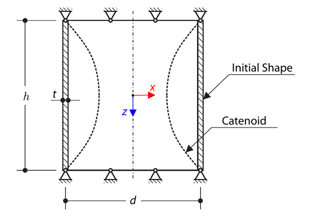
A cylindrical membrane is stretched by means of isotropic prestress. Find the final minimal shape of the membrane - catenoid. Determine the maximum radial deflection of the membrane. The add-on module RF-FORM-FINDING is used for this purpose. Elastic deformations are neglected both in RF-FORM-FINDING and in the analytical solution; self-weight is also neglected in this example.
A cable is loaded by means of a uniform load. This causes the deformed shape in the form of the circular segment. Determine the equilibrium force of the cable to obtain the given sag of the cable. The add-on module RF-FORM-FINDING is used for this purpose. Elastic deformations are neglected both in RF-FORM-FINDING and in the analytical solution; self-weight is also neglected in this example.
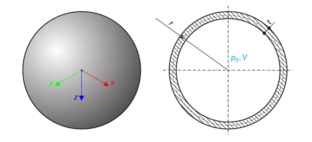
A spherical balloon membrane is filled with gas with atmospheric pressure and defined volume (these values are used for FE model definition only). Determine the overpressure inside the balloon due to the given isotropic membrane prestress. The add-on module RF-FORM-FINDING is used for this purpose. Elastic deformations are neglected both in RF-FORM-FINDING and in the analytical solution; self-weight is also neglected in this example.
An ASTM A992 W-shaped member is selected to carry a dead load of 30.000 kips and a live load of 90.000 kips in tension. Verify the member strength using both LRFD and ASD.
Consider an ASTM A992 W 18×50 beam forspan and uniform dead and live loads as shown in Figure 1. The member is limited to a maximum nominal depth of 18 inches. The live load deflection is limited to L/360. The beam is simply supported and continuously braced. Verify the available flexural strength of the selected beam, based on LRFD and ASD.
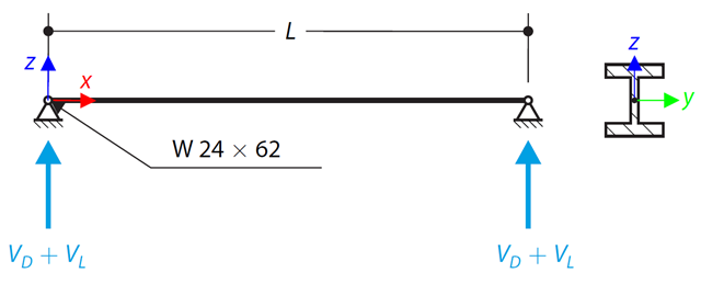
An ASTM A992 W 24×62 beam with end shears of 48.000 and 145.000 kips from the dead and live loads, respectively, is shown in Figure 1. Verify the available shear strength of the selected beam, based on LRFD and ASD.
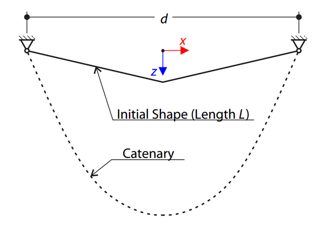
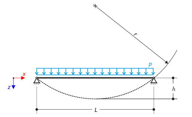
A very stiff cable is suspended between two supports. Determine the equilibrium shape of the cable (the catenary), consider the gravitational acceleration, and neglect the stiffness of the cable. Verify the position of the cable at the given test points.
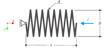
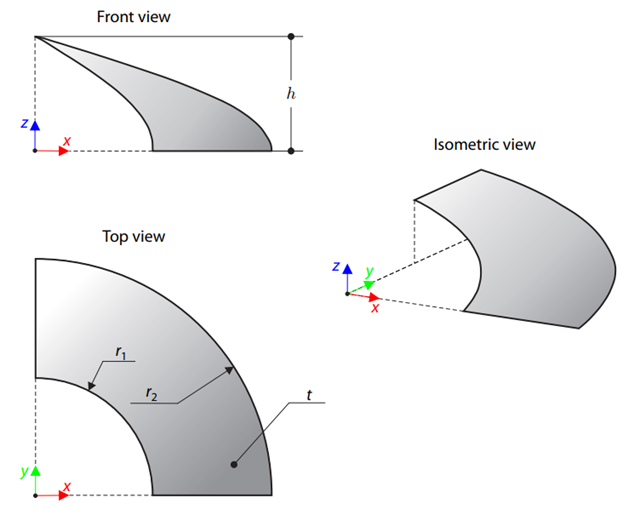
A closely coiled helical spring is loaded by a compression force. The spring has middle diameter D, wire diameter d, and it consists of i turns. The total length of the spring is L. Determine the total deflection of the spring for the member model and one‑turn deflection for the solid model.
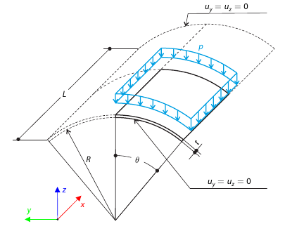
A shell roof structure under pressure load is modeled where the straight edges are free, while at the curved edges the y- and z‑translations are constrained. Neglecting self‑weight, compute the maximum (absolute) vertical deflection, and compare the results with COMSOL Multiphysics 4.3.