16 Results
View Results:
Sort by:

Question
When defining material as "Isotropic Masonry 2D", I get an error message saying the authorization of the program failed.
Question
How can I consider a door lintel made of sectional steel in my wall surface?
Question
When using plastic material, should I perform the calculation according to the second-order or large deformation analysis?
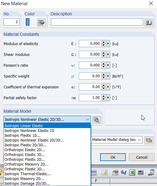
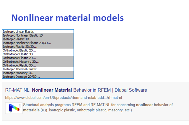
RF-MAT NL Add-on Module
I have purchased the add-on module RF‑MAT NL, but I cannot find it anywhere.
Question
How does the license distribution work for the RF‑MAT NL add‑on module in the case of a network dongle?
Question
Is it possible to perform a seismic analysis with the masonry material model?