


by Mahyar Kazemian, Sajad Nikdel, Mehrnaz Mohammad Esmaeili, Vahid Nik, Kamyab Zandi
ABSTRACT
Environmental loads, such as wind and river flow, play an essential role in the structural design and structural assessment of long-span bridges. Climate change and extreme climatic events are threats to the reliability and safety of the transport network.
This has led to a growing demand for digital twin models to investigate the resilience of bridges under extreme climate conditions. Kalix bridge, constructed over the Kalix river in Sweden in 1956, is used as a testbed in this context.
The bridge structure, made of post-tensioned concrete, consists of five spans, with the longest one being 94 m. In this study, aerodynamic characteristics and extreme values of numerical wind simulation such as surface pressure are obtained by using Spalart-Allmaras Delayed Detached Eddy Simulation (DDES) as a hybrid RANS-LES turbulence approach which is both practical and computationally efficient for near-wall mesh density imposed by the LES method.
Surface wind pressure is obtained for three extreme climate scenarios, including extreme windy weather, extremely cold weather, and design value for a 3000-year return period. The result indicates significant differences in surface wind pressure due to time layers coming from transient wind flow simulation. In order to assess the structural performance under the critical wind scenario, the highest value of surface pressure for each scenario is considered.
Also, a hydrodynamic study is conducted on the bridge pillars, in which the river flow is simulated using the VOF method, and the water movement process around the pillars is examined transiently and at different times. The surface pressure applied by the river flow with the highest recorded volumetric flow is calculated on each of the pier surfaces.
In simulating the river flow, information and weather conditions recorded in the past periods have been used. The results show that the surface pressure at the time when the river flow hit the pillars is much higher than in subsequent times. This amount of pressure can be used as a critical load in fluid-structure interaction (FSI) calculations.
Finally, for both sections, the wind surface pressure, the velocity field with respect to auxiliary probe lines, the water circumferential motion contours around the pillars, and the pressure diagram on them are reported in different timesteps.
1. Introduction
Transport infrastructures are the backbone of our society, and bridges are the bottleneck of the transport network [1]. Moreover, Climate change resulting in higher deterioration rates and extreme climatic events are important threats to the reliability and safety of transport networks. Over the last decade, many bridges have been damaged and failed by extreme weather conditions such as typhoons and floods.
Wang et al. analyzed the impacts of climate change and showed that the deterioration of concrete bridges is expected to become even worse than today, and extreme climatic events are predicted to be more often and with higher severity [2].
In addition, the demand for load-carrying capacity often increases over time, for instance, due to the use of heavier lorries for timber transportation in North Europe and North America. Thus, there is a growing need for reliable methods to assess the structural resilience of the transport network under extreme climate conditions accounting for future climate change scenarios.
Road transport assets are designed, built, and operated, relying on numerous data sources and various models. Hence, Design engineers use established models provided by standards; construction engineers
document the data on actual material and provide as-built drawings; operators collect data on traffic, carry out inspections and plan for maintenance; climate scientists combine climate data and models to
predict future climatic events, and assessment engineers compute the impact of extreme climate loading on the structure.
Given the overwhelming sources for and the complexity of data and models, the most current information and updated computations may not be readily available for crucial decisions, e.g., regarding structural safety and operability of infrastructure during episodes of extreme events. The lack of seamless integration between infrastructure data, structural models, and decision-making at system levels is a major limitation of current solutions, which leads to inadaptability and uncertainties and creates costs and inefficiencies.
Structural Digital Twin of infrastructure is a living structural simulation that brings all the data and models together and updates itself from multiple sources to represent its physical counterpart. The structural Digital Twin, maintained throughout the life cycle of an asset and easily accessible at any time, provides the infrastructure owner/users with an early insight into the potential risks to mobility induced by climatic events, heavy vehicle loads, and even aging of a transport infrastructure.
In an ongoing project, we are developing and implementing a structural digital twin for the Kalix bridge in Sweden. The overarching goal of the current paper is to present a method for and study the results of quantifying structural loads resulting from extreme climate events based on future climate scenarios for the Kalix bridge. Kalix bridge, constructed over the Kalix river in Sweden in 1956, is made of a post-tensioned concrete box girder. The bridge is used as a testbed for the demonstration of state-of-the-art assessment and structural health monitoring (SHM) methods.
The specific objective of the current research is to account for climate parameters such as wind and water flow, imposing static and dynamic loads on the structures. Our method, in the first step, consists of wind flow simulations and water flow simulations using transient CFD modeling based on the LES/DES turbulence model to quantify wind and hydro loads; this makes up the primary focal point of this paper.
In the next step, the structural response of the bridge will be studied by transforming the wind and hydro load profiles to structural loads in nonlinear structural FE analysis. Last, the structural model will be updated by seamlessly incorporating SHM data and thus creating a structural digital twin reflecting the true response of the structure. The former two research focuses remain outside the immediate scope of the current paper.
2. Kalix Bridge Description
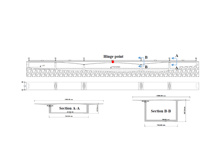
Kalix bridge consists of 5 long spans that the longest one is around 94 meters, and the shortest is 43.85 m. The bridge is made of post-tensioned concrete, which is cast in-situ segmentally and a non-prismatic box girder that is shown in Image 1. The bridge is symmetrical in geometry, and there is a hinge in the midpoint of it. The width of the bridge deck at the top and bottom slab is approximately 13 m and 7.5 m, respectively. The thickness of the wall is 45 cm, and the thickness of the bottom slab varies from 20 cm to
50 cm.
3. Wind Simulation
Wind tunnel tests used to be the only way to examine the reaction of bridges to wind loads [3]; these experiments however are time consuming and expensive. Near 6 to 8 weeks are required to conduct a typical wind tunnel test [4]. The latest achievements in the computational capacity of computers provide opportunities for practical simulation of wind around bridges using computational fluid dynamics (CFD).
It is beneficial to investigate wind pressure on bridge components using computer simulation. Simulation parameters of the bridge and the wind field around it need to be determined; therefore, their impacts on the forces applied on the bridge can be evaluated accurately.
The design demands on bridge structures require a robust investigation of wind action, especially in extreme weather conditions. Guaranteeing the stability of long-span bridges, since their features and formations are most prone to wind load, is among the main design considerations [3].
3.1. Simulation Parameters
The basic wind speed is chosen 22 m/s based on the wind map of Sweden and the location of Kalix bridge according to EN 1991-1-4 [5], and the Swedish code BFS 2019:1 EKS 11; see Image 1. The free surface above the water is considered as an exposed area for the wind load. The dominant wind attack direction is considered perpendicular to the bridge deck.
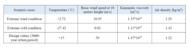
The current simulations are based on three scenarios which include: extreme wind, extreme cold, and design value for a 3000-year return period. Each condition has different values of temperature, basic wind
speed, kinematic viscosity, and air density, as shown in Table 1. The weather data sets were synthesized for two extreme weather weeks over the 30-year period of 2040-2069, considering 13 different future climate scenarios with different global climate models (GCMs) and representative concentration pathways (RCPs).
One extreme cold week and one extreme windy week were selected using the approach developed
by Nik [7]. The approach was adapted to the needs of this work, considering the weekly time scale instead of monthly. The application of the approach has been verified for complex simulations, including energy systems [7] [8], hydrothermal [9], and microclimate simulations [10].
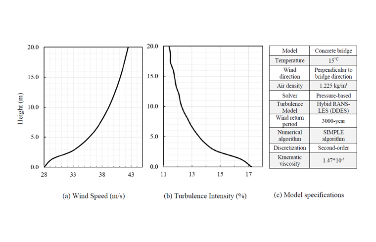
For considering the extreme weather condition of highly important infrastructure, the value of basic wind speed needs to be transferred from 50-year return period to 3000-year as stated in equation 1 [6]. The velocity and turbulence profile is created based on EN 1991-1-4 [5] for terrain category 0 (Z0 = 0.003 m and Zmin = 1 m), where Z0 and Zmin are roughness length and minimum height, respectively. The variation of wind speed with height is defined in Equation 2, where co(z) is orography factor taken as 1, vm(z) is mean wind velocity at the height z, kr is terrain factor depending on the roughness length, and Iv(z) is the turbulence intensity; see Equation 3.
The value of wind speed for T = 3000-year return period is calculated to be 31 m/s; thus, the wind speed and turbulence intensity diagrams are obtained as shown in Image 2.
3.2. Turbulence Model
To make the investigations accurate on the flow around important structures such as bridges, a hybrid approach including delayed detached-eddy simulations (DDES) is applicable and computationally efficient [11] [12]. This turbulence model uses a RANS method near the boundary layers and the LES method far from the boundary layers and in the separated region's area of the flow.
In the first step, the detached-eddy simulation approach has been extended to acquire reliable force predictions on the models with a great impact of separated flow. There are various examples in the review part of Spalart [11] for several cases which use the application of the detached-eddy simulation (DES) turbulence model.
The initial DES formulation [13] is developed by using Spalart–Allmaras approach. Regarding the transition from RANS to LES approach, the term of destruction in the modified viscosity transport equation is revised: the distance between a point in the domain and the nearest solid surface (d) is substituted with the factor introduced by:
where CDES is a coefficient, it is considered as 0.65 and Δ is a length scale associated with local grid spacing:
A modified approach of DES, known as delayed detached-eddy simulation (DDES), has been employed to dominate the probable problem of “grid-induced separation” (GIS) which is related to the grid geometry. The objective of this new approach is to confirm that the turbulence modeling keeps in RANS mode throughout the boundary layers [14]. Therefore, the definition of the parameter is modified as defined:
where fd is a filter function that a value of 0 is considered in near-wall boundary layers (RANS zone) and a value of 1 in areas where the flow separation took place (LES zone).
3.3. Computational Grid and Results
RWIND 2.01 Pro is employed for CFD wind simulation, which uses external CFD code OpenFOAM® version 17.10. Three-dimensional CFD simulation is performed as a transient wind simulation for incompressible turbulent flow using SIMPLE (Semi-Implicit Method for Pressure Linked Equations) algorithm.
In the current simulation, the steady-state solver is considered as the initial condition which means when the transient flow is being calculated, the steady-state computation of the initial condition starts in the first part of the simulation, and as soon as it is completed, the transient calculation will start automatically.
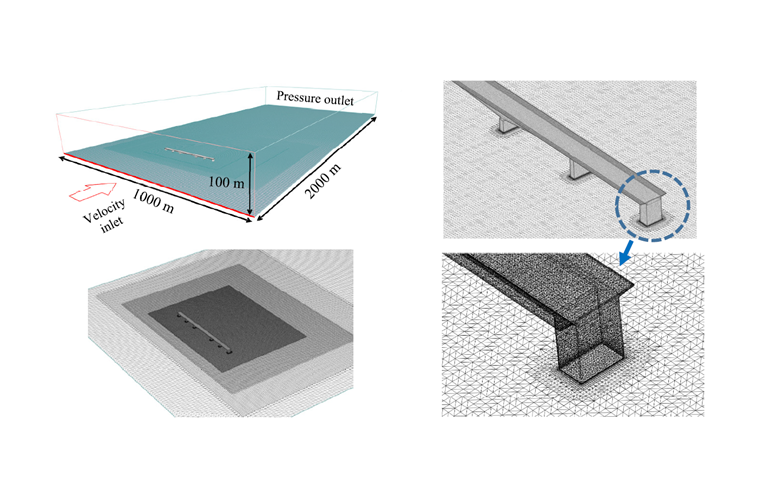
The computational grid is performed by a three-dimensional 8,057,279 cells and 8,820,901 nodes, also the wind tunnel domain dimensions are considered 2000 m * 1000 m * 100 m (length, width, height) as shown in Image 3. The minimum cell volume is 6.34*10-5 m3, the maximum volume is 812.30 m3 and the maximum skewness is 1.80.
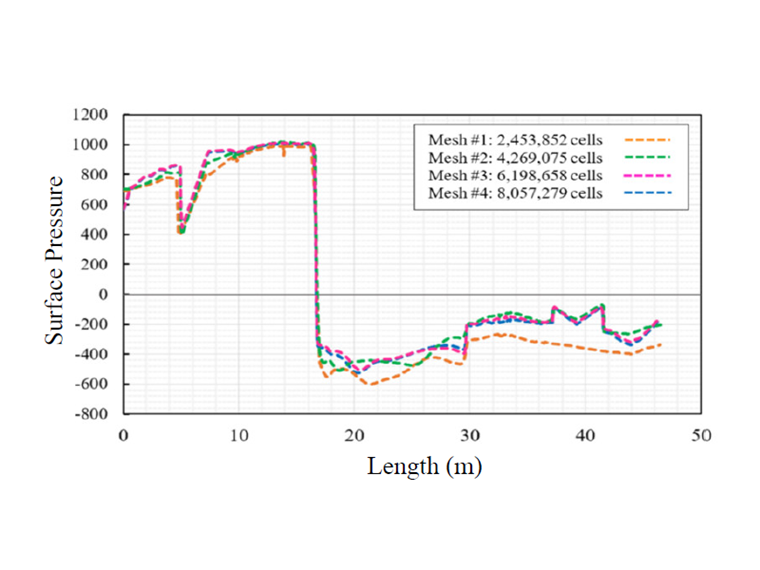
The final residual pressure is considered 5*10-5. The process of mesh generation and grid independency has been carried out using four mesh sizes that are shown in Image 4 for the reference mesh, and finally, the grid independency has achieved.
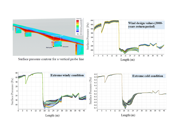
Three simulations have been performed to obtain the wind pressure value for extreme weather conditions and design wind value that is shown in Image 5. For each scenario, the result of wind pressure is obtained by using the transient DDES turbulence model with respect to 30 (s) duration that includes 60-time layers (Δt=0.5 s).
It can be observed that the front area of the bridge is exposed to positive wind pressure and the amount of pressure is increasing by the height near the edge of the deck for all scenarios. Also, Image 5. illustrates the negative wind pressure values entirely on the deck surface. The value belonging for the 3000-year period is much higher than the other scenarios.
It is important to note that the range of the input wind speed has a great impact on the value of the surface pressure rather than the other parameters. In addition, for each scenario, the higher range of wind pressure and suction during total time needs to be considered as critical wind load imposed on the structure. The lowest value of surface pressure is obtained in the extreme cold condition scenario while in the extreme windy condition, the value of pressure becomes one order of magnitude higher.
In addition, it is important to note that the performance of the bridge completely would be different due to different air temperatures, and a possible critical case can occur in the scenario that experiences lower pressure. Regarding the input value of each scenario, the highest range of wind pressure belongs to the design level due to the 3000-year return period, which has received the highest wind speed as input velocity.
4. Hydro Simulation
Bridge pillars across the river can block the flow by reducing the river’s cross-section, creating local eddy currents, and changing the flow velocity, which may put pressures on the pillar surfaces. When the river flows into the bridge pillars, the process of flowing water around the base can be divided into two parts: applying pressure at the time when water hits the bridge pillar, and after the initial pressure when the water flows around the pillars [15].
When the water reaches the bridge pillars at a certain velocity, the effect of the pressure on the pillars is much greater than the pressure of the fluid remaining around them. Due to the developments of computer science as well as the increasing development of computational fluid dynamic codes, various numerical simulations have been widely used, and it has been proven that the results of many simulations are consistent with experimental results [16].
Accordingly, in this research, the computational fluid dynamics method has been used to simulate the phenomena governing river flow behavior. A three-dimensional solution based on numerical calculations using the LES turbulence model has been selected for this study. Three-dimensional simulation of river flow in different directions and velocities allows us to calculate and analyze all the pressures on the surface of bridge pillars at different time intervals.
4.1. Simulation Parameters
The river flow can be defined as a two-phase flow, including water and air, in an open channel. Open channel flow is a fluid flow with a free surface on which the atmospheric pressure is evenly distributed and is created by the weight of the fluid. To simulate this type of flow, VOF multi-phase method is used.
The commercially available program Flow3D uses VOF and FAVOF volumetric-fraction methods. In the VOF method, the modeling domain is first divided into cells of smaller elements or volumes of controls. For fluid-containing elements, numerical values are held for each of the flow variables inside them.
These values represent the volumetric average of the values in each element. In free surface currents, all cells are not full of fluid; some cells on the flow surface are half full. In this case, a quantity called volume of fluid, F, is defined representing the part of the cell that is filled by the fluid.
After determining the position and angle of the flow surface, it will be possible to apply the appropriate boundary conditions at the flow surface to calculate the fluid motion. As the fluid moves, the value of F also changes with it. Free surfaces are automatically monitored by the movement of fluid within a fixed network. The FAVOR method is used to determine the geometry.
Another volumetric-fraction quantity can also be used to determine the level of an unoccupied rigid body (Vf). When the volume occupied by the rigid body in each cell is known, the fluid boundary within the fixed network can be determined like VOF. This boundary is used to determine the boundary conditions of the wall that the stream follows. In general, the equation of mass continuity is as follows:
Motion equations for fluid velocity components in 3D coordinates, or in another word the Navier-Stokes equations, are as follows:
Where VF is the open volume ratio to flow, ρ is the fluid density, (u, v, w) are the velocity components in x, y, and z-direction, respectively, RSOR is the source function, (Ax, Ay, Az) are the fractional areas, (Gx, Gy, Gz) are the gravitational forces, (fx, fy, fz) are the viscosity accelerations, and (bx, by, bz) are the flow losses in porous media in x, y, and z-direction, respectively [17].
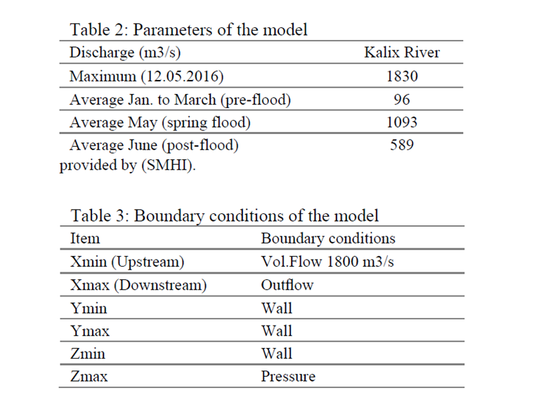
The catchment area of the Kalix River is large and wide, so it has a sub-polar climate with cold and long winters and mild and short summers. About 50% of the rainfall in this area is snow. In May, usually, snow melting causes a significant increase in river discharge. The climatic conditions of the river are summarized in Table 2, [18].
Contrary to the general trend of this study, the mentioned weather conditions forecast is using the weather information recorded in the past periods. Based on the available weather information, we defined the boundary conditions when performing the calculations.
4.2.Computational Ggrid and Results
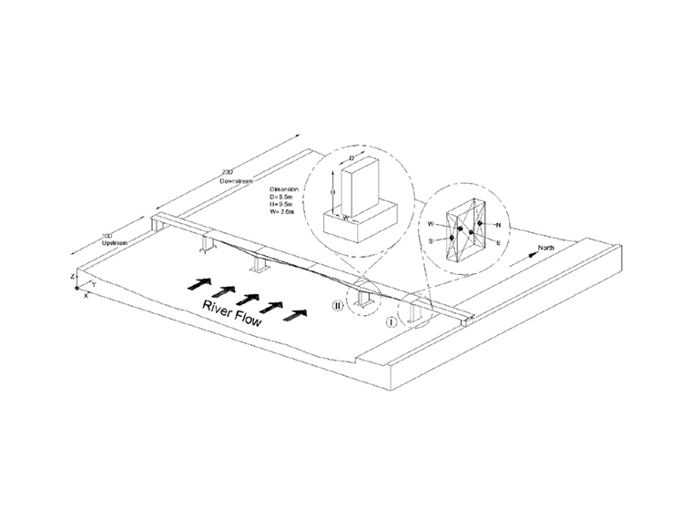
First, according to the dimensions of the columns in three directions X, Y, Z, and according to the longitudinal dimension of the pillars (D = 8.5 m; see Image 7), the domain extends by 10D upstream and by 20D downstream. Structured meshing method (Cartesian) and Flow3D software have been used to solve this problem. For a correct grid, the domain must be divided into different sections.
This division is based on places with strong gradients. Using the creation of a new surface, the domain can be divided into several sections to create a regular mesh with correct and appropriate dimensions, the number of cells on each surface can be specified.
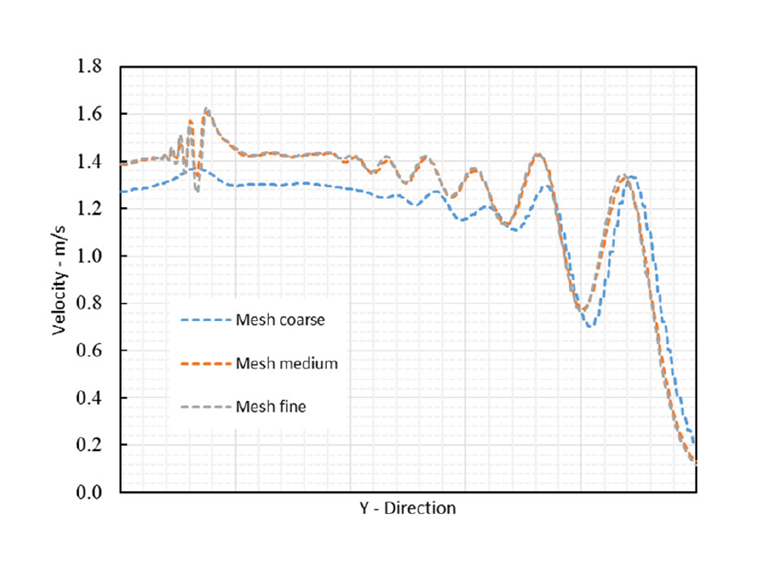
This increases the final volume of the cells. For this reason, we have meshed this domain into three levels: Coarse, medium, and fine. The results of grid independence studies are given in Image 6. To check the calculated results, we must first make sure that the input current is correct. To do this, the input flow rate is measured to the solution domain and compared with the base value. The dimensions of the solution domain are specified in Image 7. This image also contributes to the recognition of the bridge pillars and their surface naming.
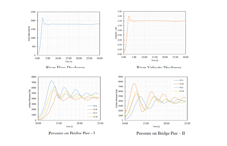
As it is shown in Image 8, the river flow is within the allowable range for 90% of the simulation time, and the inlet flow rate has been simulated correctly. Besides, in Image 9, the average velocity of the river is calculated based on the flow rate as well as the cross-sectional area of the river.
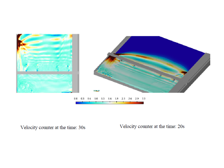
To extract the amount of pressure applied to the different sides of the columns, we have selected the simulation time interval from 10 to 25 seconds (discharge stabilization time in the amount of 1800 cubic meters per second). The calculated results for each side are shown in Image 10 and 11. Velocity contours are also shown in Images 12 and 13. These contours are adjusted based on the fluid velocity at a given time.
Due to the dimensions of the solution domain and the flow rate of the river, the water flow reaches the bridge pillars in the tenth second and the initial pressure of the river flow affects the surfaces of the bridge pillars. This initial pressure decreases over time and is stabilized in a certain range for each side according to the area and the percentage of interaction with the flow. For Fluid-structure interaction (FSI) calculations, the calculated critical pressure at the time when the current strikes the pillars can be used.
5. Conclusion
The effects of extreme weather conditions, including dynamic wind and water flow, were investigated numerically for the Kalix bridge. Three scenarios were defined for dynamic wind simulations including extreme windy weather, extreme cold weather, and design value for a 3000-year return period. Leveraging CFD simulations, wind pressures within 60-time steps (30 seconds) were determined using the transient DDES turbulence model.
The results indicate significant differences between the scenario implying the importance of input data especially the wind velocity diagram. It was observed that the design value for the 3000-year return period has much higher impact than the other scenarios. Furthermore, it was shown the importance of considering the higher range of surface wind pressure through time steps to assess the structural performance of the bridge in the most critical condition.
Besides, the maximum river flow was considered for a transient simulation according to the recorded weather conditions, and bridge pillars were subjected to the maximum river flow for 30 seconds. Hence, besides the river flow physical conditions and how the flow direction changes in downstream, maximum water pressures were quantified at the time when the flow hits the pillars.
In the future work, the structural performance of Kalix bridge will be evaluated by
imposition wind load, water pressure, as well as traffic load, thus creating a structural digital twin reflecting the true response of the structure.
6. Acknowledgement
The authors greatly appreciate the support of Dlubal Software for providing RWIND Simulation license, as well as Flow Sciences Inc. for providing FLOW-3D license.
Authors
Mahyar Kazemian, PhD candidate, intern at the Department of Engineering, Timezyx Inc., Canada.
Sajad Nikdel, M.Sc. student, intern at the Department of Engineering, Timezyx Inc., Canada.
Mehrnaz Mohammad Esmaeili, Bachelor student, intern at the Department of Engineering, Timezyx Inc., Canada.
Vahid Nik, Associate Professor at the division of Building Physics, Lund University, and Chalmers University of Technology, Sweden.
Kamyab Zandi, Director, Timezyx Inc., Vancouver, BC V6N 2R2, Canada. Email: [email protected].
