Introduction
When a complicated structure is designed and experimental data of wind-induced pressures on surfaces are available, it is possible to apply them in static analysis using RFEM 6 and RWIND 2.
First, data from pressure probes must be defined on the model in their locations. This is possible either in RFEM 6 or directly in the RWIND stand-alone program (as verification data): see Technical Article 1870 .
The definition gives the program discrete information about the pressures. However, the pressure values must somehow be distributed on the structure surfaces in order to enable wind load calculation and static analysis. This is performed by RWIND 2. The CFD calculation runs in the background in order to create an appropriate mesh and to enable the verification of experimental data (however, when only static analysis from the measured data is performed, the CFD calculation results are not important, and a convergence is not needed).
Note that the interpolation is not based on real physical phenomena and its credibility strongly depends on the number (or density) of pressure probes. However, even from a limited number of pressure probes, a pressure distribution can be suggested and its quality depends on the engineering knowledge of the user. Remember that these interpolation methods are just a tool to distribute pressure on the surface, without respect to physical phenomena.
Workflow in RWIND 2
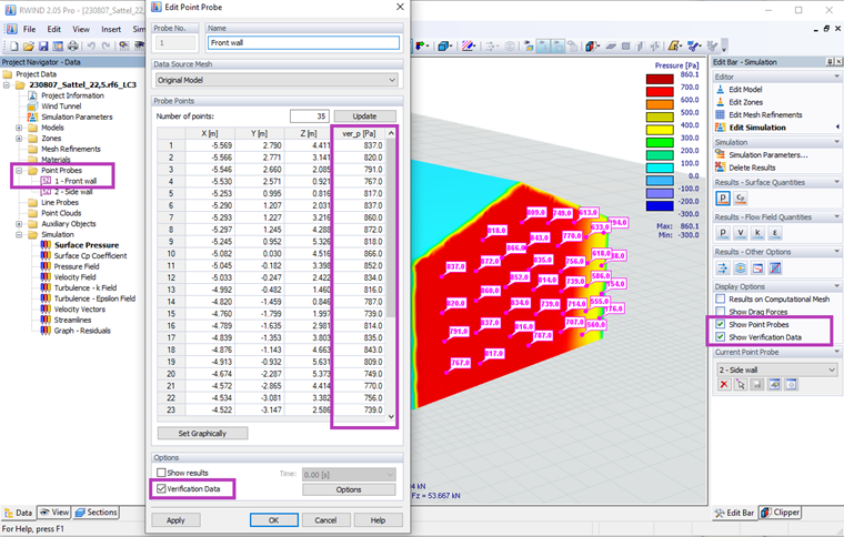
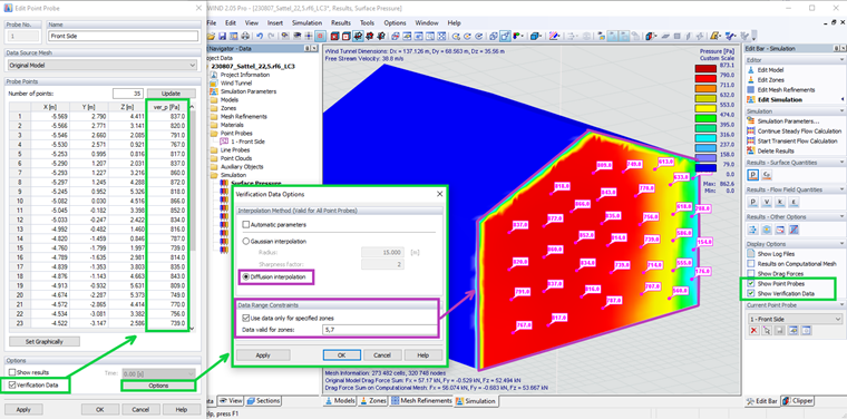
First, define the point probes on your model. In RWIND 2, you can define several points in one point probe. This is suitable when all points have the same properties (zone constraint, and so on). The probes on original model are suitable for the experimental data. Check the "Verification Data" option and define the measured pressures in the "ver_p" column (Image 01).
Zone Constraint
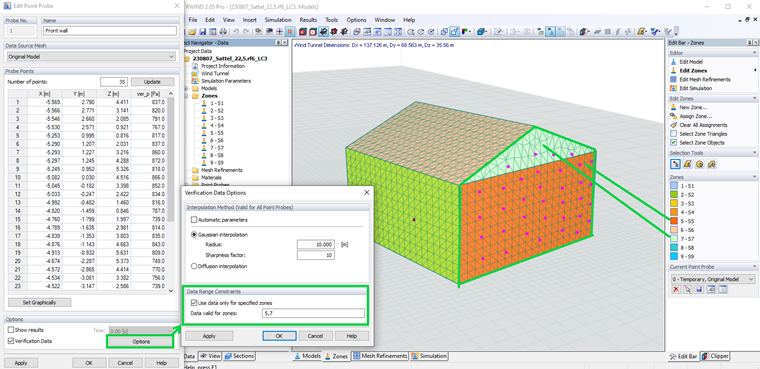
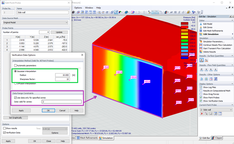
Wind-induced pressure is significantly dependent on wind direction. It is obvious that this pressure differs strongly according to surface orientation to the wind. It is, therefore, useful to constrain the pressure interpolation on a specific surface. In RWIND, each probe can be constrained to one or more specific zones (Image 02).
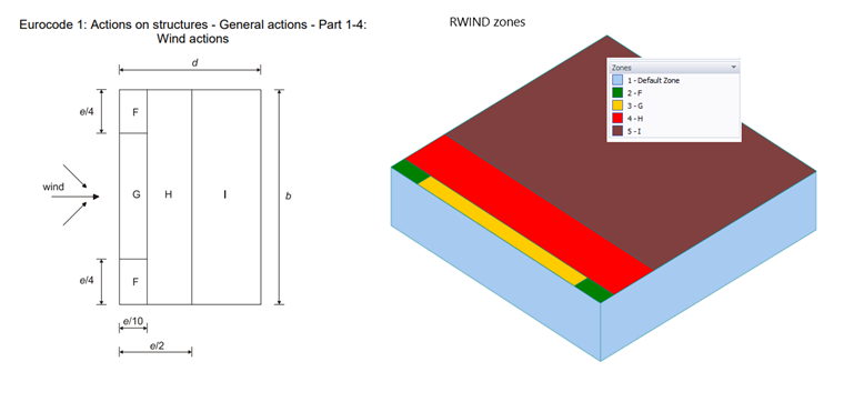
The zones must be defined before the calculation. Several zones can be created on one surface, that is, in a way similar to the standard suggestions for simple structures (Image 03) or according to a preliminary CFD calculation.
Interpolation Methods
Two interpolation methods are available in RWIND: diffusion interpolation and Gaussian interpolation kernel. Only one method must be selected for all probes.
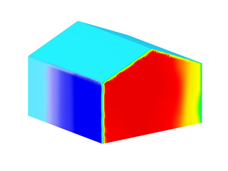
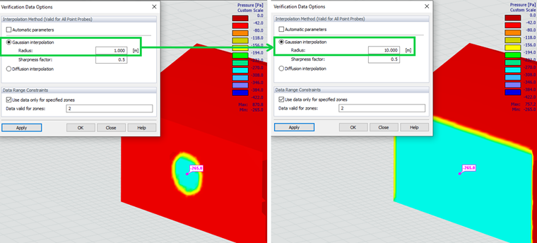
The diffusion method distributes the data from the "source" point over the surface. It is suitable for dense mesh of measuring points (Image 04). In the case of thin open structures, this method interpolates values only on one side of the plate. The method is dependent on the mesh density.
On the other hand, the Gaussian interpolation kernel interpolates the values around the "source" in 3D. Therefore, it is not suitable for thin open structures, because it influences both sides of the surface. For closed structures (buildings, and so on), this method works well (Image 05).
The Gaussian method parameters control the resulting distribution.
The radius sets how far the "source" influences the surrounding area. If the radius is greater than the constraint zone, a nearly constant distribution can be created from one probe (Image 06). On the other hand, when the radius is greater than the distance between the probes and a low sharpness factor is used, the resulting value in the relevant probe is influenced by the neighboring probe.
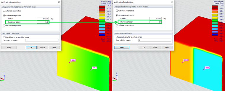
The sharpness factor controls the steepness of the transition between probes. Higher factors create sharper borders (Image 07).
Conclusion
The interpolation of experimental data enables the application of measured wind-induced pressures in static analysis. The experimental values can be defined either in RFEM 6 or directly in RWIND 2. The interpolation methods are not based on a physical principle, while CFD is. They are only tools to interpolate the measured values. The more measured values you define, the better accordance with the reality you can reach.