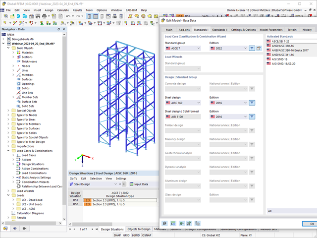
The design of cold-formed steel members according to the AISI S100-16 / CSA S136-16 is available in RFEM 6. Design can be accessed by selecting “AISC 360” or “CSA S16” as the standard in the Steel Design Add-on. “AISI S100” or “CSA S136” is then automatically selected for the cold-formed design.
RFEM applies the Direct Strength Method (DSM) to calculate the elastic buckling load of the member. The Direct Strength Method offers two types of solutions, numerical (Finite Strip Method) and analytical (Specification). The FSM signature curve and buckling shapes can be viewed under Sections.
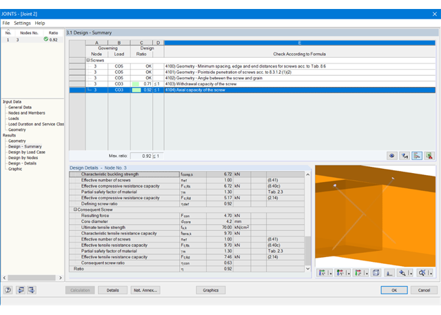
At first, the governing joint designs are arranged in groups and displayed with the basic geometry of the joint in the first result window. In the other result windows, you can see all fundamental design details.
Dimensions, material properties, and welds important for the connection construction are displayed immediately and can be printed directly. Similarly, export to DXF-file is enabled. The connections can be visualized in the RF-/JOINTS Timber - Timber to Timber module as well as in RFEM/RSTAB.
All graphics can be included in the RFEM/RSTAB printout report or printed directly. Due to the scaled output, an optimal visual check is possible as early as in the design phase.
The following design results are displayed:
- Check of minimum spacing
- Load-carrying capacity of each screw
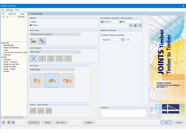
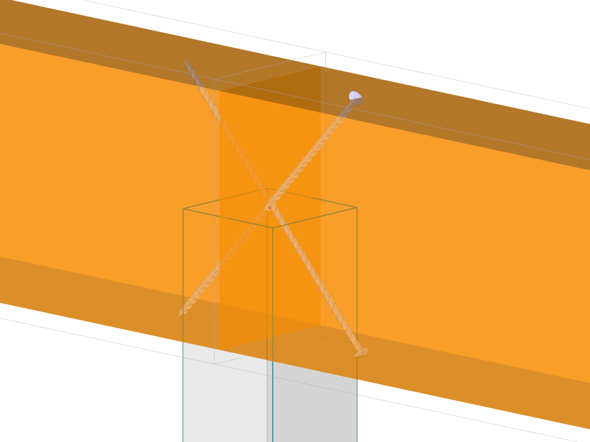
First, select the joint type and the design standard.
The connected members are imported from the RFEM/RSTAB model. The add-on module automatically checks if all geometry conditions are fulfilled.
In addition, the loads are imported automatically from RFEM/RSTAB. In the Geometry window, you can specify the screw parameters (diameter, length, angle, and so on).
.png?mw=640&hash=c1087880acc023575381bb136280b0c348568350)
- Design of hinged connections
- Biaxial inclination of the connected member (for example, a jack rafter joint)
- Connection of any number of members on one node for the type "Main member only"
- Screw diameter 6 mm – 12 mm
- Automatic check of the minimum distance between screws
- Optional free definition of screw distances
- Transfer of eccentricity from RFEM/RSTAB
- Crosswise or parallel screw alignment
- Definition of up to 16 screws in a row
- Graphical visualization of joints in the add-on module and in RFEM/RSTAB
- Performing all required designs
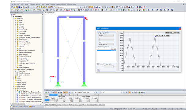
Due to the integration of RF‑/DYNAM Pro in RFEM or RSTAB, you can incorporate numeric and graphic results from RF‑/DYNAM Pro - Nonlinear Time History to the global printout report. Also, all RFEM and RSTAB options are available for a graphical visualization. The results of the time history analysis are displayed in a time history diagram.
The results are displayed as a function of time and the numerical values can be exported to MS Excel. Result combinations can be exported, either as a result of a single time step or the most unfavorable results of all time steps are filtered out.
Calculation in RFEM
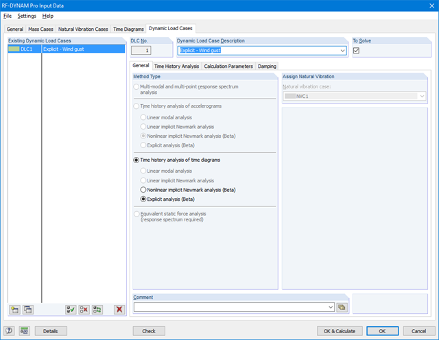
The nonlinear time history analysis is performed with the implicit Newmark analysis or the explicit analysis. Both are direct time integration methods. The implicit analysis requires small time steps to provide precise results. The explicit analysis determines the required time step automatically to provide the stability to the solution. The explicit analysis is suitable for the analysis of short excitations, such as impulse excitation, or an explosion.
Calculation in RSTAB
The nonlinear time history analysis is performed with the explicit analysis. This is a direct time integration method and determines the required time step automatically in order to provide the solution stability.
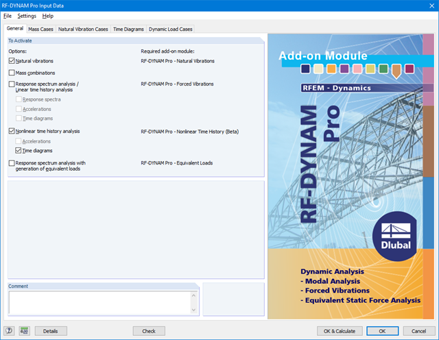
RF-/DYNAM Pro - Nonlinear Time History is integrated in the structure of RF‑/DYNAM Pro - Forced Vibrations and extended by two nonlinear analysis methods (one nonlinear analysis in RSTAB).
Force-time diagrams can be entered as transient, periodic, or as a function of time. Dynamic load cases combine the time diagrams with the static load cases, which provides high flexibility. Furthermore, it is possible to define time steps for the calculation, structural damping, and export options in the dynamic load cases.

- Nonlinear member types, such as tension and compression members or cables
- Member nonlinearities, such as failure, tearing, yielding under tension or compression
- Support nonlinearities, such as failure, friction, diagram, and partial activity
- Release nonlinearities, such as friction, partial activity, diagram, and fixed if positive or negative internal forces
.png?mw=640&hash=8cfd0c4bd093c03de543d147ffbf6f5c9250634a)
- User-defined time diagrams as a function of time, in tabular form, or as harmonic loads
- Combination of the time diagrams with RFEM/RSTAB load cases or combinations (enables definition of nodal, member, and surface loads, as well as free and generated loads varying over time)
- Combination of several independent excitation functions
- Nonlinear time history analysis with the implicit Newmark analysis (RFEM only) or the explicit analysis
- Structural damping using Rayleigh damping coefficients or Lehr's damping
- Direct import of initial deformations from a load case or combination (RFEM only)
- Stiffness modifications as initial conditions; for example, axial force effect, deactivated members (RSTAB only)
- Graphical display of results in a time history diagram
- Export of results in user-defined time steps or as an envelope
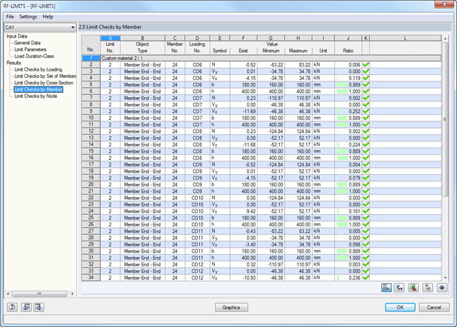
First, the governing design checks of the connection for the respective load case, and load combination, or result combination are displayed. In addition, it is possible to display results separately for sets of members, surfaces, cross-section, members, nodes, and nodal supports.
- You can use a filter to further reduce the displayed results and thus present them in a clearer way.
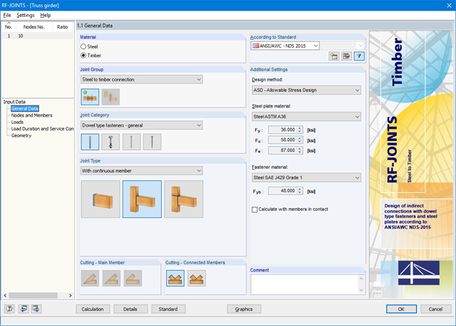
First, it is necessary to select the joint type, design standard, and steel plate and dowel material. For design according to EN 1995-1-1, you can select the SFS intec dowel system WS‑T. In this case, the corresponding material is preset in accordance with the technical approval of the manufacturer.
The connected members are imported from the RFEM/RSTAB model. The add-on module automatically checks if all geometry conditions are fulfilled. Alternatively, you can define the connection manually.
- The loading is also imported from RFEM/RSTAB or, in the case of manual joint definition, loads are entered. The Geometry window includes steel plate dimensions and fastener layouts.
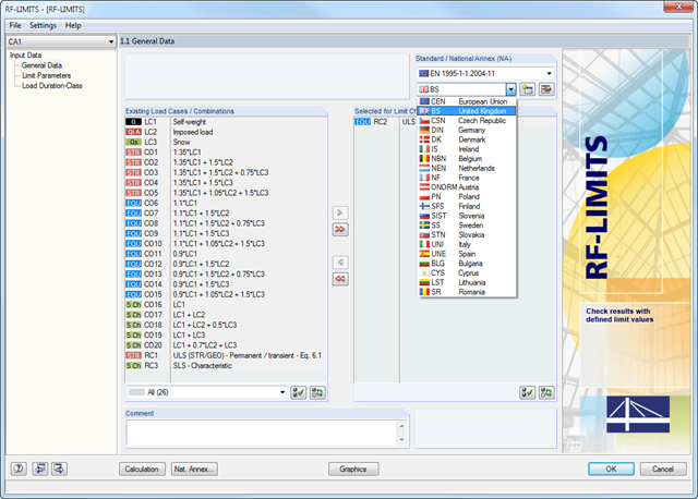
After selecting the loads required for the design and, if necessary, the desired standard for the design, you can define the limit loads in Window 1.2 Limit Parameters. In addition to the manufacturers listed in the limit library, it is possible to add user-defined entries.
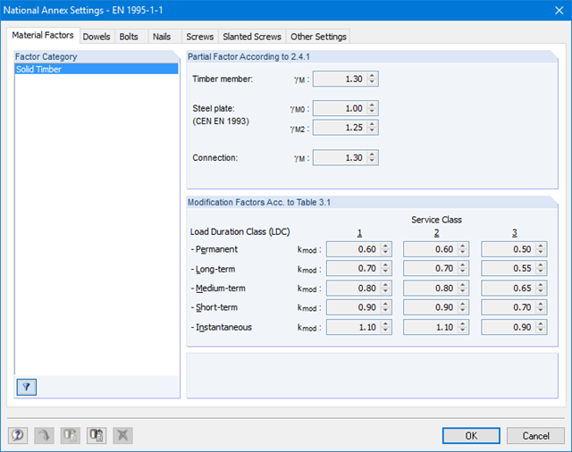
After selecting all limit elements for the design, you can optionally define the load duration class (LDC). However, this module window is available only for timber fastener design according to EN 1995-1-1 or DIN 1052.
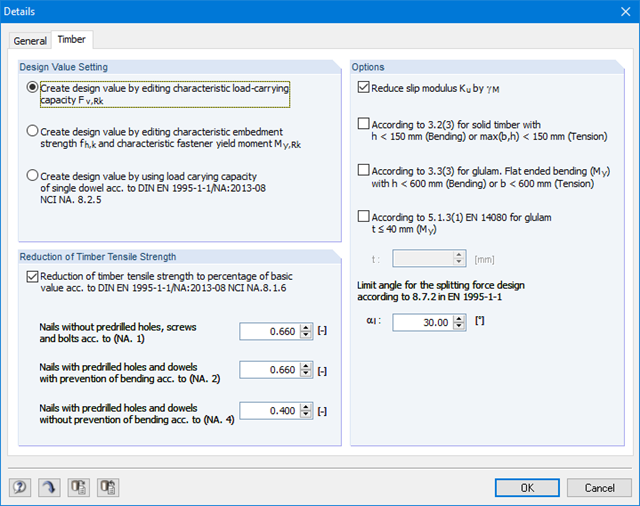
After the calculation, the RF‑/JOINTS Timber - Steel to Timber add‑on module lists joint stiffnesses of all individual members, among other things. The following design results are displayed:
- Check of minimum spacing
- Load-carrying capacity of single fastener
- Steel plates (bearing resistance and stress according to EC 3 and AISC)
- Stress analysis with reduced timber cross‑section
- Block shear failure
- Total load carrying-capacity (including stiffness determination, transversal tension design according to EC 5, and others)
- Fire resistance design according to EN 1995‑1‑2
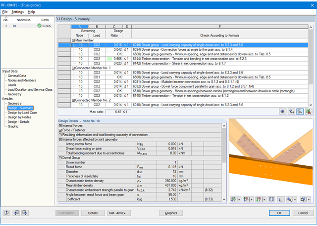
At first, the governing joint designs are arranged in groups and displayed with the basic geometry of the joint in the first result window. In the other result windows, you can see all fundamental design details.
Dimensions, material properties, and welds important for the connection construction are displayed immediately and can be printed directly. Similarly, export to DXF-file is enabled. It is possible to visualize the connections in RF‑/JOINTS Timber - Steel to Timber or in the RFEM/RSTAB model.
All graphics can be included in the RFEM/RSTAB printout report or printed directly. Due to the scaled output, an optimal visual check is possible as early as in the design phase.
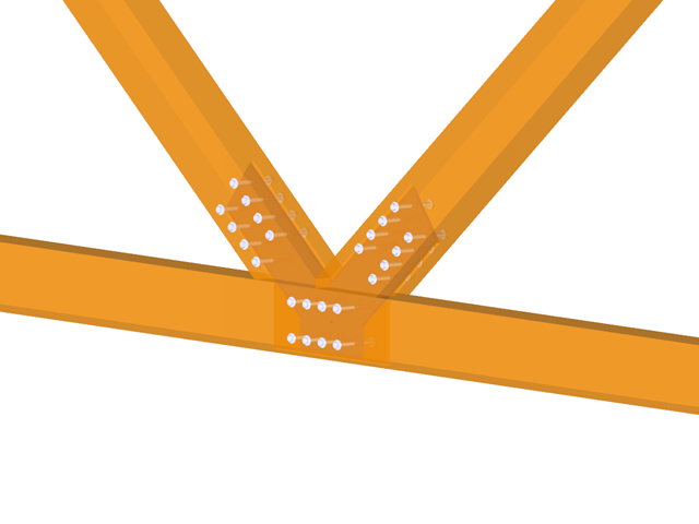
- Design of hinged, bending resistant, and semi-rigid connections
- Definition of up to 5 steel plates slotted in timber beams
- Up to 8 members connected to one node
- Thickness of steel plate 5 mm – 40 mm
- All sizes of fasteners
- Automatic check of the minimum distance between fasteners
- Optional free definition of fastener distances
- Definition of asymmetrical fastener arrangements (for example, any polygonal chains)
- Graphical visualization of joints in the add-on module and in RFEM/RSTAB
- All required steel and timber designs, including reduction of cross‑section values
- Design of transversal tension reinforcement (for EN 1995‑1‑1 only)
- Export of the member eccentricities to RFEM/RSTAB to be considered in the determination of internal forces
- Dowel length optionally shorter than cross-section width (for wooden plugs)
- DXF Export of Connection Geometry
- Fire resistance design according to EN 1995‑1‑2
- Design of member ends, members, nodal supports, nodes, and surfaces
- Consideration of specified design areas
- Check of cross-section dimensions
- Design according to EN 1995-1-1 (European Timber Standard) with the respective National Annexes + DIN 1052 + DSTV DIN EN 1993-1-8 + ANSI / AWC - NDS 2015 (US Standard)
- Design of various materials, such as steel, concrete, and others
- No necessary linking to specific standards
- Extensible library including timber fasteners (SIHGA, Sherpa, WÜRTH, Simpson StrongTie, KNAPP, PITZL) and steel fasteners (standardized connections in steel building design according to EC 3, M-connect, PFEIFER, TG-Technik)
- Ultimate load capacities of timber beams by the companies STEICO and Metsä Wood available in the library
- Connection to MS Excel
- Optimization of connecting elements (the most utilized element is calculated)