
If there is a load case or load combination in the program, the stability calculation is activated. You can define another load case in order to consider initial prestress, for example.
For this, you need to specify whether to perform a linear or nonlinear analysis. Depending on the case of application, you can select a direct calculation method, such as the Lanczos method or the ICG iteration method. Members not integrated in surfaces are usually displayed as member elements with two FE nodes. With such elements, the program cannot determine the local buckling of single members. That's why you have the option to divide members automatically.

You can select several methods that are available for the eigenvalue analysis:
- Direct Methods
- The direct methods (Lanczos [RFEM], roots of characteristic polynomial [RFEM], subspace iteration method [RFEM/RSTAB], and shifted inverse iteration [RSTAB]) are suitable for small to medium-sized models. You should only use these fast solver methods if your computer has a larger amount of memory (RAM).
- ICG Iteration Method (Incomplete Conjugate Gradient [RFEM])
- In contrast, this method only requires a small amount of memory. Eigenvalues are determined one after the other. It can be used to calculate large structural systems with few eigenvalues.
Use the Structure Stability add-on to perform a nonlinear stability analysis using the incremental method. This analysis delivers close-to-reality results also for nonlinear structures. The critical load factor is determined by gradually increasing the loads of the underlying load case until the instability is reached. The load increment takes into account nonlinearities such as failing members, supports and foundations, and material nonlinearities. After increasing the load, you can optionally perform a linear stability analysis on the last stable state in order to determine the stability mode.

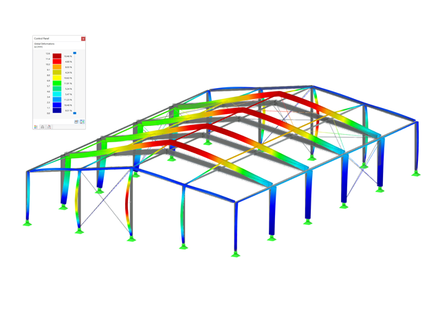
As the first results, the program presents you with the critical load factors. You can then perform an evaluation of stability risks. For member models, the resulting effective lengths and critical loads of the members are displayed to you in tables.
Use the next result window to check the normalized eigenvalues sorted by node, member, and surface. The eigenvalue graphic allows you to evaluate the buckling behavior. This makes it easier for you to take countermeasures.

- Calculation of models consisting of member, shell, and solid elements
- Nonlinear stability analysis
- Optional consideration of axial forces from initial prestress
- Four equation solvers for an efficient calculation of various structural models
- Optional consideration of stiffness modifications in RFEM/RSTAB
- Determination of a stability mode greater than the user-defined load increment factor (Shift method)
- Optional determination of the mode shapes of unstable models (to identify the cause of instability)
- Visualization of the stability mode
- Basis for determining imperfection
- A wide range of available sections, such as rolled I-sections; channel sections; T-sections; angles; rectangular and circular hollow sections; round bars; symmetrical and asymmetrical, parametric I-, T-, and angle sections; built-up cross-sections (suitability for design depends on the selected standard)
- Design of general RSECTION cross-sections (depending on the design formats available in the respective standard); for example, equivalent stress design
- Design of tapered members (design method depending on the standard)
- Adjustment of the essential design factors and standard parameters is possible
- Flexibility due to detailed setting options for basis and extent of calculations
- Fast and clear results output for an immediate overview of the result distribution after the design
- Detailed output of the design results and essential formulas (comprehensible and verifiable result path)
- Numerical results clearly arranged in tables and graphical display of the results in the model
- Integration of the output into the RFEM/RSTAB printout report
- Design of tension, compression, bending, shear, torsion, and combined internal forces
- Tension design with consideration of a reduced section area (for example, hole weakening)
- Automatic classification of cross-sections to check local buckling
- Internal forces from the calculation with Torsional Warping (7 DOF) are taken into account by means of the equivalent stress check (currently not yet for the design standard ADM 2020).
- Design of cross-sections of Class 4 with effective cross-section properties according to EN 1993‑1‑5 (licenses for RSECTION and Effective Sections are required for the RSECTION cross-sections)
- Shear buckling check with consideration of transverse stiffeners

- Stability analyses for flexural buckling, torsional buckling, and flexural-torsional buckling under compression
- Lateral-torsional buckling analysis of the structural components subjected to moment loading
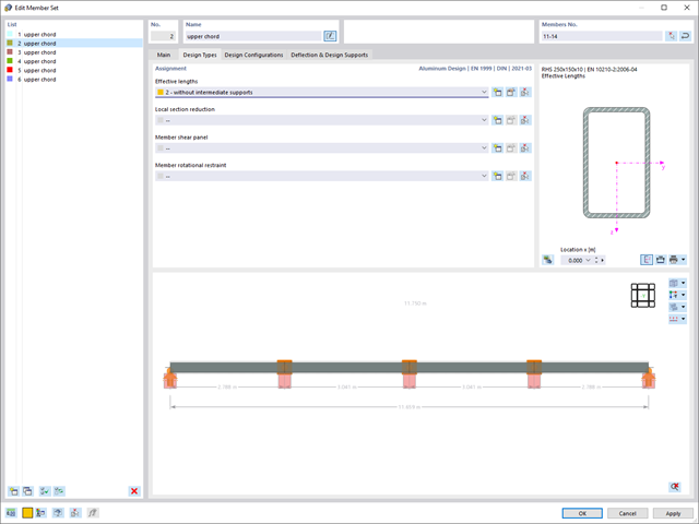
- Import of the effective lengths from the calculation using the Structure Stability add-on
- Graphical input and check of the defined nodal supports and effective lengths for stability analysis
- Depending on the standard, a choice between user-defined input of Mcr, analytical method from the standard, and use of internal eigenvalue solver
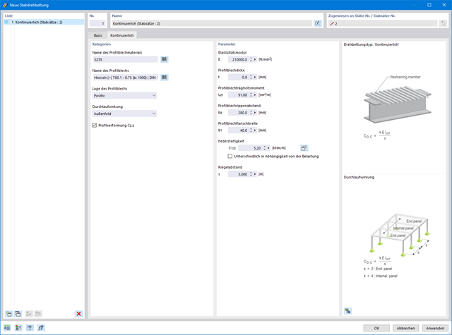
- Consideration of a shear panel and a rotational restraint when using the eigenvalue solver
- Graphical display of a mode shape if the eigenvalue solver was used
- Stability analysis of structural components with the combined compression and bending stress, depending on the design standard
- Comprehensible calculation of all necessary coefficients, such as interaction factors
- Alternative consideration of all effects for the stability analysis when determining internal forces in RFEM/RSTAB (second-order analysis, imperfections, stiffness reduction, possibly in combination with the Torsional Warping (7 DOF) add-on)

- Realistic representation of interaction between a building and soil
- Realistic representation of the influences of the foundation components on each other
- Extensible library of soil properties
- Consideration of several soil samples (probes) at different locations, even outside the building
- Determination of settlements and stress diagrams as well as their graphical and tabular display

Entering soil layers for soil samples is performed in a clearly arranged dialog box. A corresponding graphical representation supports clarity and makes checking the input user-friendly.
An extensible database facilitates the selection of soil material properties. The Mohr-Coulomb model as well as a nonlinear model with stress and strain dependent stiffness are available for a realistic modeling of the soil material behavior.
You can define any number of soil samples and layers. The soil is generated from all entered samples using 3D solids. Assignment to the structure is carried out using coordinates.
The soil body is calculated according to the nonlinear iterative method. The calculated stresses and settlements are displayed graphically and in tables.

The Dlubal structural analysis software does a lot of work for you. The input parameters, which are relevant for the selected standards, are suggested by the program in accordance with the rules. Furthermore, you can enter response spectra manually.
Load cases of the type Response Spectrum Analysis define the direction in which response spectra act and which eigenvalues of the structure are relevant for the analysis. In the spectral analysis settings, you can define details for the combination rules, damping (if applicable), and zero-period acceleration (ZPA).

Did you know that Equivalent static loads are generated separately for each relevant eigenvalue and excitation direction. These loads are saved in a load case of the Response Spectrum Analysis type and RFEM/RSTAB performs a linear static analysis.

The load cases of the type Response Spectrum Analysis contain the generated equivalent loads. First, the modal contributions have to be superimposed with the SRSS or CQC rule. In this case, you can use the signed results based on the dominant mode shape.
Afterwards, the directional components of earthquake actions are combined with the SRSS or the 100% / 30% rule.
Compared to the RF‑/STABILITY (RFEM 5) and RSBUCK (RSTAB 8) add-on modules, the following new features have been added to the Structure Stability add-on for RFEM 6 / RSTAB 9:
- Activation as a property of a load case or a load combination
- Automated activation of the stability calculation via combination wizards for several load situations in one step
- Incremental load increase with user-defined termination criteria
- Modification of the mode shape normalization without recalculation
- Result tables with filter option
Compared to the RF-/DYNAM Pro - Equivalent Loads add-on module (RFEM 5 / RSTAB 8), the following new features have been added to the Response Spectrum Analysis add-on for RFEM 6 / RSTAB 9:
- Response spectra of numerous standards (EN 1998, DIN 4149, IBC 2018, and so on)
- User-defined response spectra or those generated from accelerograms
- Direction-relative response spectrum approach
- Results are stored centrally in a load case with underlying levels to ensure clarity
- Accidental torsional actions can be taken into account automatically
- Automatic combinations of seismic loads with the other load cases for use in an accidental design situation
Compared to the RF‑SOILIN add-on module (RFEM‑5), the following new features have been added to the Geotechnical Analysis add-on for RFEM 6:
- Creation of the layered soil as a 3D model from the entirety of the defined soil samples
- Recognized material law according to Mohr-Coulomb for soil simulation
- Graphical and tabular output of stresses and strains at any depth of the soil
- Optimal consideration of the soil-structure interaction on the basis of an overall model
Compared to the RF‑/ALUMINUM add-on module (RFEM 5 / RSTAB 8), the following new features have been added to the Aluminum Design add-on for RFEM 6 / RSTAB 9:
- In addition to Eurocode 9, the US standard ADM 2020 is integrated.
- Consideration of the stabilizing effect of purlins and sheets by rotational restraints and shear panels
- Graphical display of the results in the gross section
- Output of the used design check formulas (including a reference to the used equation from the standard)

The stress and strain results by surface can be output in the surface result table according to the thickness layer.

Do you want to model and analyze the behavior of a soil solid? To ensure this, special suitable material models have been implemented in RFEM.
You can use the modified Mohr-Coulomb model with a linear-elastic ideal-plastic model or a nonlinear elastic model with an oedometric stress-strain relation. The limit criterion, which describes the transition from the elastic area to that of the plastic flow, is defined according to Mohr-Coulomb.

Enter and model a soil solid directly in RFEM. You can combine the soil material models with all common RFEM add-ons.
This allows you to easily analyze the entire models with a complete representation of the soil-structure interaction.
All parameters required for the calculation are automatically determined from the material data that you have entered. The program then generates the stress-strain curves for each FE element.

Did you know? You can enter the soil layers that you have obtained from the subsoil expertises done in the locations into the program in the form of soil samples. Assign the explored soil materials, including their material properties, to the layers.
For the definition of the samples, you can enter the data in tables as well as in the respective editing dialog box. Furthermore, you can also specify the groundwater level in the soil samples.