26 Wyniki
Wyświetl wyniki:
Sortuj według:

W rozszerzeniu Analiza geotechniczna dostępny jest wysokiej jakości model materiałowy "Zmodyfikowany model gruntu twardniejącego". Ten model materiałowy jest odpowiedni dla różnych gruntów i jest w stanie odpowiednio odwzorować następujące właściwości rzeczywistego gruntu.
- Zależność naprężenia od sztywności gruntu
- Zależność ścieżki obciążenia od sztywności gruntu
- Odkształcenia plastyczne jeszcze przed osiągnięciem warunku granicznego
- Wzrost wytrzymałości na ścinanie wraz ze wzrostem zagęszczenia siatki
- Wzrost granicy plastyczności wraz ze wzrostem naprężenia, aż do osiągnięcia granicznego warunku plastyczności
- Kryterium uszkodzenia według Mohra-Coulomba
Więcej informacji na temat tego modelu materiałowego oraz definicji danych wejściowych w programie RFEM można znaleźć w odpowiednim rozdziale instrukcji online rozszerzenia Analiza geotechniczna.
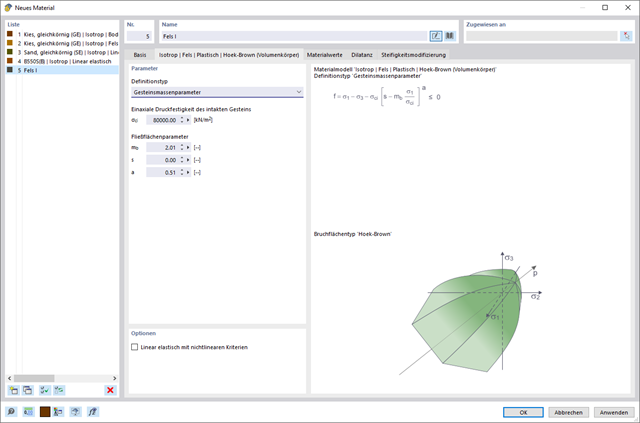
W rozszerzeniu Analiza geotechniczna dostępny jest model Hoek'a-Brown'a. Model wykazuje zachowanie materiału liniowo-sprężystego idealnie plastycznego. Jego nieliniowe kryterium wytrzymałości jest najczęściej stosowanym kryterium zniszczenia skał.
Parametry materiału można wprowadzić bezpośrednio za pomocą
- parametrów skały lub alternatywnie poprzez
- klasyfikację GSI.
opisane.
Weiterführende Informationen zu diesem Materialmodell und der Definition der Eingabe in RFEM finden Sie im entsprechenden Kapitel im Online-Handbuch für das Add-On Geotechnische Analyse: Model Hoeka-Browna .
- 002720
- Ogólne informacje
- Analiza stateczności konstrukcji RFEM 6
- Analiza stateczności konstrukcji RSTAB 9
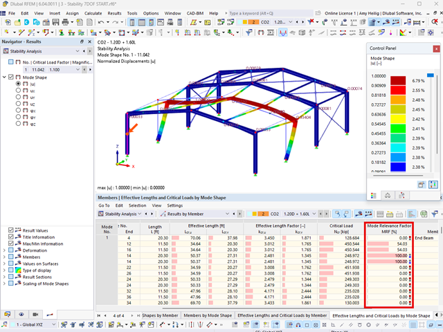
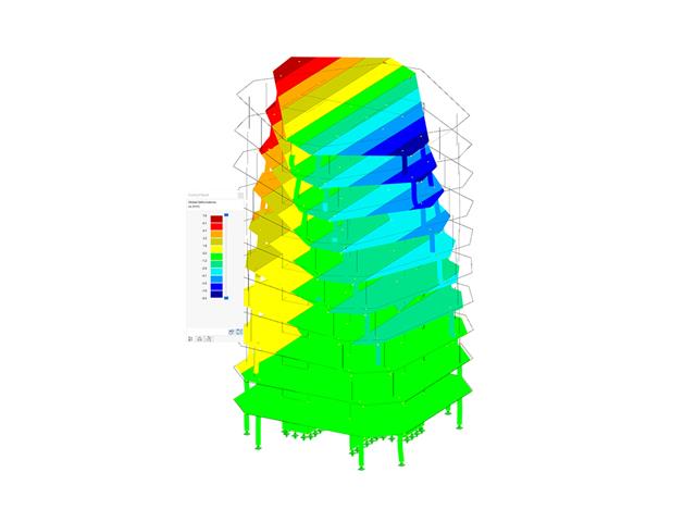
Stosując modalny współczynnik istotności (MRF) można ocenić, w jakim stopniu poszczególne elementy konstrukcyjne przyczyniają się do powstania rzeczywistego kształtu wyboczenia. Obliczenia opierają się na energii względnego odkształcenia sprężystego każdego pojedynczego pręta.
Dzięki MRF można rozróżnić lokalne i globalne kształty wyboczenia. Jeżeli kilka prętów ma znaczny MRF (np. > 20%), bardzo prawdopodobna jest niestateczność całej konstrukcji lub jej części. Jeżeli jednak suma wszystkich MRF dla kształtu drgań wynosi około 100%, należy spodziewać się lokalnego problemu ze statecznością (np. wyboczenia pojedynczego pręta).
Ponadto MRF może być wykorzystany do określenia obciążeń krytycznych i równoważnych długości wyboczeniowych poszczególnych prętów (np. do analizy stateczności). Kształty wyboczenia, dla których dany pręt ma małe wartości MRF (np. <20%), mogą zostać w tym kontekście pominięte.
MRF jest wyświetlany według kształtów wyboczenia w tabeli wyników w sekcji Analiza stateczności --> Wyniki według prętów --> Długości efektywne i obciążenia krytyczne.
.png?mw=640&hash=55038d2a1591f62179796666cb9b2fede0274e19)
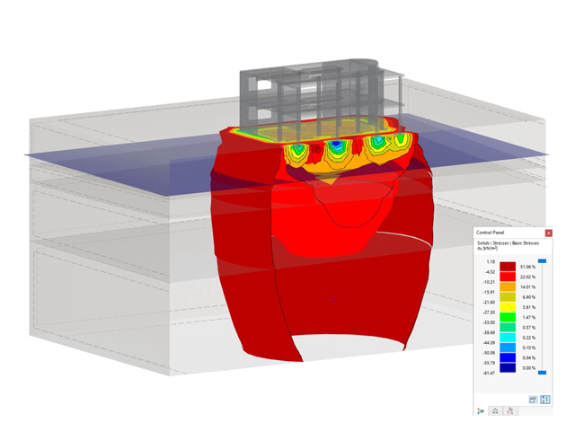
Graficzne i tabelaryczne wyświetlanie wyników dla deformacji, naprężeń i odkształceń pomaga określić bryłę gruntu. Aby to osiągnąć, skorzystaj ze specjalnych kryteriów filtrowania, które umożliwiają wybór określonych wyników.
Program na pewno cię nie zawiedzie. Jeśli chcesz graficznie ocenić wyniki w bryłach gruntu, dostępne są obiekty pomocnicze. Na przykład można zdefiniować płaszczyzny przycinania. Umożliwia to przeglądanie odpowiednich wyników na dowolnej płaszczyźnie bryły gruntu.
I nie tylko to. Wykorzystanie przekrojów wyników i brył przycinania ułatwia graficzną analizę brył gruntu.
Wiesz już, że grunt i konstrukcję można modelować i analizować w całym modelu. Oznacza to, że wyraźnie uwzględniono interakcję gleba-konstrukcja. Dostosowanie jednego elementu konstrukcyjnego prowadzi do natychmiastowego prawidłowego uwzględnienia w analizie i wynikach dla całego układu gruntu i konstrukcji.
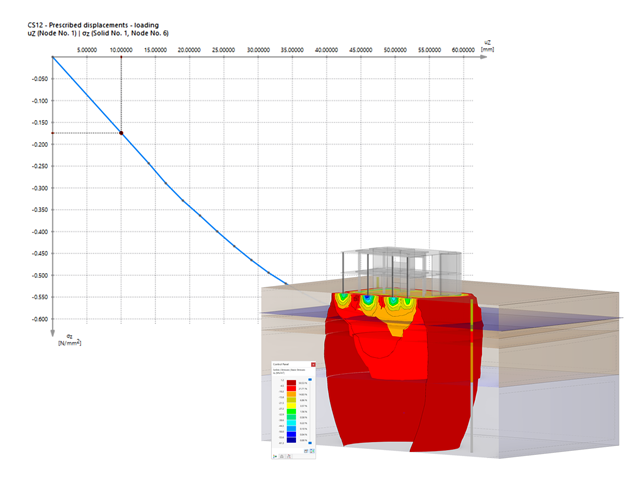
Czy jesteś gotowy na ocenę? Skorzystaj z wykresów obliczeniowych, które pokazują rozkład określonego wyniku podczas obliczeń.
Przypisanie osi pionowej i poziomej wykresu obliczeniowego można dowolnie definiować. Umożliwia to np. wyświetlenie przebiegu osiadania określonego węzła w zależności od obciążenia.
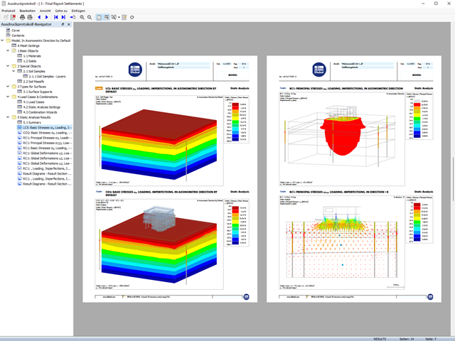
Twoje dane są zawsze dokumentowane w wielojęzycznym raporcie. W każdej chwili możesz dostosować treść i zapisać ją jako szablon. W raporcie można również za pomocą kilku kliknięć umieścić grafiki, teksty, wzory MathML i dokumenty PDF.
Wprowadzenie i modelowanie bryły gruntowej bezpośrednio w programie RFEM. Modele materiałów gruntowych można łączyć ze wszystkimi popularnymi rozszerzeniami dla programu RFEM.
Umożliwia to łatwą analizę całych modeli z pełną prezentacją interakcji grunt-konstrukcja.
Wszystkie parametry wymagane do obliczeń są określane automatycznie na podstawie wprowadzonych danych materiałowych. Następnie program generuje krzywe naprężenie-odkształcenie dla każdego elementu ES.
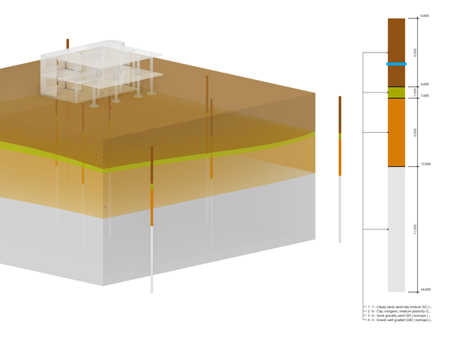
Czy wiecie, że...? Uwarstwienie gruntu, pobrane z raportów o podłożu gruntowym w miejscach wychodni, można wprowadzić bezpośrednio do programu w postaci próbek gruntu. Przypisz badane materiały gruntowe wraz z ich właściwościami do warstw.
Za pomocą danych tabelarycznych i okna dialogowego edycji można zdefiniować próbkę. Można również określić poziom wód gruntowych w próbkach gruntu.
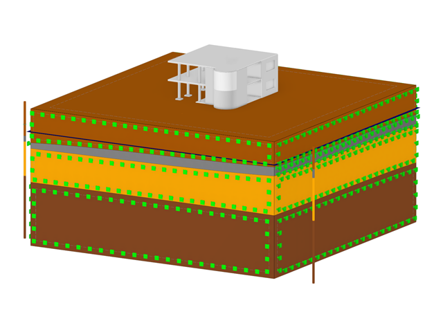
Bryły gruntu, które mają zostać przeanalizowane, są sumowane w masywach gruntu.
Próbki gruntu należy wykorzystać jako podstawę do zdefiniowania masywu gruntowego. W ten sposób program umożliwia generowanie masywu w sposób przyjazny dla użytkownika, w tym automatyczne określanie granic faz na podstawie danych z próbki, a także poziomu wód gruntowych i podpór powierzchni granicznej.
Masywy gruntowe umożliwiają określenie docelowego rozmiaru siatki ES niezależnie od ustawień globalnych dla reszty konstrukcji. Dzięki temu w całym modelu można uwzględnić różne wymagania dotyczące budynku i gruntu.
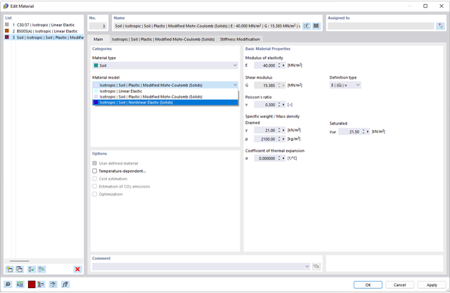
Czy chcesz modelować i analizować zachowanie bryły gruntowej? Aby to zapewnić, w programie RFEM zaimplementowano odpowiednie modele materiałowe.
Można użyć zmodyfikowanego modelu Mohra-Coulomba z liniowo-sprężystym modelem idealnie plastycznym lub nieliniowo sprężystym modelem z edometryczną relacją naprężenie-odkształcenie. Kryterium graniczne, które opisuje przejście od obszaru sprężystości do obszaru płynięcia plastycznego, jest zdefiniowane według Mohra-Coulomba.

Dzięki rozszerzeniu Analiza historii czasowej (TDA) można uwzględnić zmienne w czasie zachowanie materiału w przypadku prętów i powierzchni. Długotrwałe efekty, takie jak pełzanie, skurcz i starzenie, mogą wpływać na rozkład sił wewnętrznych, w zależności od konstrukcji. Darauf bereiten Sie sich mit diesem Add-On optimal vor.
Dla każdego przypadku obciążenia można wyświetlić odkształcenia w czasie końcowym.
Wyniki te są również dokumentowane w protokole wydruku programów RFEM i RSTAB. Zawartość protokołu i jego zakres można wybrać specjalnie dla poszczególnych warunków projektowych.

- 002165
- Ogólne informacje
- Skręcanie skrępowane (7 stopni swobody) RFEM 6
- Skręcanie skrępowane (7 stopni swobody) RSTAB 9
W porównaniu z modułem dodatkowym RF-/STEEL Warping Torsion (RFEM 5/RSTAB 8) do rozszerzenia Skręcanie skrępowane (7 DOF) dla programu RFEM 6/RSTAB 9 dodano następujące nowe funkcje:
- Pełna integracja ze środowiskiem RFEM 6 i RSTAB 9
- Siódmy stopień swobody jest bezpośrednio uwzględniany w obliczeniach prętów w programie RFEM/RSTAB na całym układzie
- Nie ma już potrzeby definiowania warunków podparcia lub sztywności sprężystej do obliczeń w uproszczonym układzie zastępczym
- Możliwość łączenia z innymi rozszerzeniami, na przykład do obliczania obciążeń krytycznych dla wyboczenia skrętnego i zwichrzenia z analizą stateczności
- Brak ograniczeń dla stalowych przekrojów cienkościennych (możliwe jest również obliczenie momentu krytycznego, na przykład dla belek o masywnych przekrojach drewnianych)

W porównaniu z modułem dodatkowym RF-SOILIN (RFEM 5) do rozszerzenia Analiza geotechniczna dla programu RFEM 6 dodano następujące nowe funkcje:
- Tworzenie warstwowego gruntu jako modelu 3D z całości zdefiniowanych próbek gruntu
- Symulacja gruntu zgodnie z teorią Mohra-Coulomba
- Graficzne i tabelaryczne przedstawienie naprężeń i odkształceń na dowolnej głębokości gruntu
- Optymalne uwzględnienie interakcji gruntu i konstrukcji na podstawie modelu ogólnego
- 002162
- Ogólne informacje
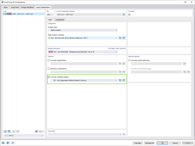
- Analiza stateczności konstrukcji RFEM 6
- Analiza stateczności konstrukcji RSTAB 9
W porównaniu z modułami dodatkowymi RF-STABILITY (RFEM 5) i RSBUCK (RSTAB 8) do rozszerzenia Stateczność konstrukcji dla programu RFEM 6/RSTAB 9 dodano następujące nowe funkcje:
- Aktivierung als Eigenschaft eines Lastfalls oder einer Lastkombination
- Automatisierte Aktivierung der Stabilitätsberechnung über Kombinationsassistenten für mehrere Lastsituationen in einem Schritt
- Inkrementelle Laststeigerung mit benutzerdefinierten Abbruchkriterien
- Veränderung der Eigenformnormierung ohne Neuberechnung
- Ergebnistabellen mit Filteroption
_ENG.png?mw=640&hash=1053c9bef400e9f5361c9c3278f76a272fcc4ddf)
Czy aktywowałeś rozszerzenie Analiza historii czasowej (TDA)? Dobrze, teraz można dodawać dane czasowe do przypadków obciążeń. Po zdefiniowaniu początku i końca obciążenia, uwzględniany jest wpływ pełzania na końcu obciążenia. Program umożliwia modelowanie efektów pełzania w konstrukcjach szkieletowych i kratowych wykonanych z betonu zbrojonego.
W tym przypadku obliczenia są przeprowadzane nieliniowo zgodnie z modelem reologicznym (model Kelvina i Maxwella).
Czy obliczenia zakończyły się pomyślnie? Wyznaczone siły wewnętrzne można teraz wyświetlić w tabelach i grafice, a także uwzględnić w obliczeniach.
- Realistyczne odwzorowanie interakcji między budynkiem a gruntem
- Realistyczne odwzorowanie oddziaływania poszczególnych fundamentów na siebie nawzajem
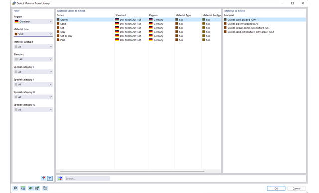
- Biblioteka parametrów gruntowych z możliwością rozszerzania
- Możliwość uwzględniania wielu próbek gruntu z różnych lokalizacji, także poza obrysem budynku
- Określanie osiadań oraz wykresów naprężeń w gruncie oraz ich prezentacja w formie graficznej i tabelarycznej
Wprowadzanie warstw gruntu dla potrzeb zadawania próbek gruntu odbywa się w przejrzystym oknie dialogowym. Odpowiadająca temu prezentacja graficzna zapewnia przejrzystość i ułatwia kontrolę wprowadzanych danych.
Rozszerzalna baza danych ułatwia wybór właściwości materiałowych dla gruntu. Dla realistycznego odwzorowania zachowania się materiału gruntowego można użyć modelu Mohra-Coulomba oraz model gruntu ze wzmocnieniem.
Można zdefiniować dowolną liczbę próbek i warstw gruntu. Grunt jest odwzorowany na podstawie wszystkich wprowadzonych próbek za pomocą brył 3D. Przypisanie do konstrukcji odbywa się za pomocą współrzędnych.
Zachowanie bryły gruntu jest obliczane za pomocą nieliniowej metody iteracyjnej. Obliczone naprężenia i osiadania są wyświetlane graficznie oraz w tabelach.
- 002073
- Ogólne informacje
- Analiza stateczności konstrukcji RFEM 6
- Analiza stateczności konstrukcji RSTAB 9
- Obliczanie modeli składających się z elementów prętowych, powłokowych i bryłowych
- Nieliniowa analiza stateczności
- Możliwość uwzględniania sił osiowych od wstępnego sprężenia
- Cztery dostępne solvery do rozwiązywania równań dla efektywnego obliczania różnych modeli konstrukcyjnych
- Opcjonalne uwzględnianie zmian w sztywności w programie RFEM/RSTAB
- Wyszukiwanie postaci wyboczeniowych o krytycznym mnożniku obciążenia większym niż zadany przez użytkownika (metoda "przesunięcia")
- Możliwość określania wektorów własnych dla modeli niestatecznych (w celu zidentyfikowania przyczyny niestateczności)
- Wizualizacja postaci niestateczności
- Podstawa określania imperfekcji