Properties and Calculation of Result Values of Line Supports

Calculation of Support Forces

First, it must be clear how the result of a line support is determined. A line support is internally divided into nodal supports at each mesh point. The program then determines the support force for each nodal support. The linear distribution between the individual (nodal) support points is created by means of certain smoothing options taking into account the influence of adjacent supports. This result corresponds to the actual distribution.

If you take a square plate with constant loading on both sides as a simple example, you can already see that the number of finite elements as well as the used stiffness of the plate (thickness, Poisson's ratio, isotropic, or orthotropic) and the stiffness of the support play a major role.

Example 1: Constant Surface Load

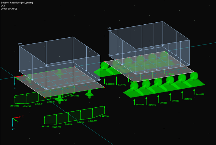
A 20-cm-thick slab with the dimensions 2 × 2 m and an FE mesh width of 40 cm is loaded by a surface load of 3 kN/m². Poisson's Ratio was assumed to be 0. The model was entered a second time with nodal supports.

The distribution of the line support forces is ascertained with the determined nodal support reactions, influence width, and smoothing option. At the edge points, the influence width corresponds to 20 cm (= half FE mesh width) and inside 40 cm (= entire FE mesh width).

K1 = 0.488678 → L1 = 0.488678/0.2 = 2.44339 kN/m
K2 = 1.325770 → L2 = (1.325770 · 3 + 1.185550) / 4 / 0.4 = 3.2267875 kN/m
K3 = 1.185550 → L3 = (1.185550 · 2 + 1.325770 + 1.185550) / 4 / 0.4 = 3.0515125 kN/m
K4 = 1.185550 → L4 = (1.185550 · 2 + 1.185550 + 1.325770) / 4 / 0.4 = 3.0515125 kN/m
K5 = 1.325770 → L5 = (1.325770 · 3 + 1.185550) / 4 / 0.4 = 3.2267875 kN/m
K6 = 0.488678 → L6 = 0.488678 / 0.2 = 2.44339 kN/m

Example 1

Example 2: Additional Nodal Support

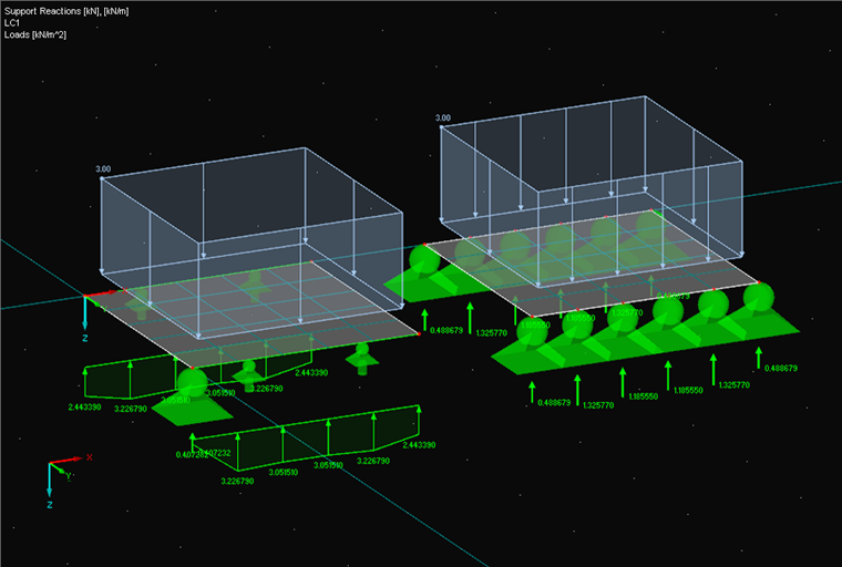
Like Example 1, but an additional nodal support is inserted at the beginning of the line support. A corresponding warning message is displayed before the calculation. Apart from the additionally supported node, there are no differences. Since the total load at Node 1 must be the value from the example above and both supports have the same stiffness, it results in the following value for both the nodal support and the initial coordinate of the line support.

K1 = L1
K1 + 0.2 · K1 = 0.751475 → K1 = 0.488678 / 1,2 = 0.4072317 kN and kN/m

Example 2

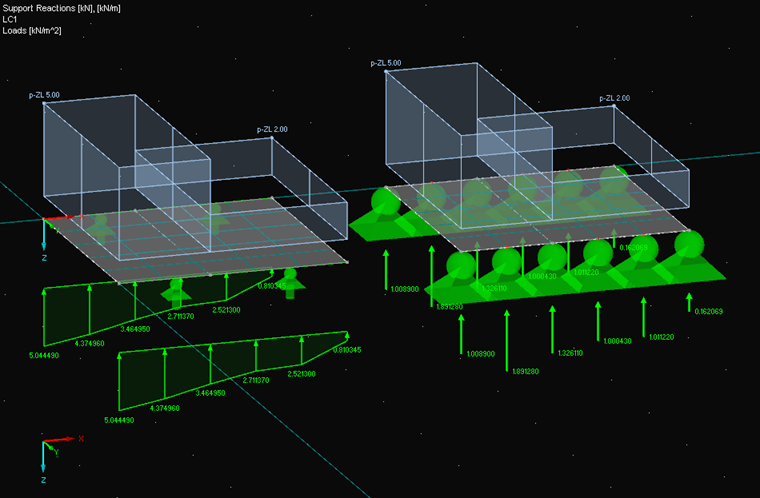
Example 3: Two Different Block Loads

K1 = 1.008900 → L1 = 1.008900 / 0.2 = 5.044500 kN/m
K2 = 1.891280 → L2 = (1.891280 · 3 + 1.326110) / 4 / 0.4 = 4.374969 kN/m
K3 = 1.326110 → L3 = (1.326110 · 2 + 1.891280 + 1.000430) / 4 / 0.4 = 3.464956 kN/m
K4 = 1.000430 → L4 = (1.000430 · 2 + 1.326110 + 1.011220) / 4 / 0.4 = 2.711369 kN/m
K5 = 1.011220 → L5 = (1.011220 · 3 + 1.000430) / 4 / 0.4 = 2.521306 kN/m
K6 = 0.162069 → L6 = 0.162069 / 0.2 = 0.810345 kN/m

Example 3

Example 4 Linear Smoothing with Example 3

The program must determine a trapezoid that has the same integral and the same centroid coordinates as the displayed polygonal chain. The roughness of the FE mesh is less important for determining the surface (corresponds to the load sum), but it is very important for determining the coordinates of the centroid. Additionally, the inclination of the smoothed gradient must follow the ordinates of the actual gradient. It is similar to the linear trend line calculation in Excel. First, the integrals of the individual partial areas are determined.

A1 = (5.044500 + 4.374969) / 2 · 0.4 = 1.8838938 kN
A2 = (4.374969 + 3.464956) / 2 · 0.4 = 1.5679850 kN
A3 = (3.464956 + 2.711369) / 2 · 0.4 = 1.2352650 kN
A4 = (2.711369 + 2.521306) / 2 · 0.4 = 1.0465350 kN
A5 = (2.521306 + 0.810345) / 2 · 0.4 = 0.6663302 kN

Sum of support forces of line = 6.400009 kN

The local centroids of the individual partial areas are:

xs1 = 0.4 / 3 · ((5.044500 + 2 · 4.374969) / (5.044500 + 4.374969)) = 0.195261366 m
xs2 = 0.4 / 3 · ((4.374969 + 2 · 3.464956) / (4.374969 + 3.464956)) = 0.192261724 m
xs3 = 0.4 / 3 · ((3.464956 + 2 · 2.711369) / (3.464956 + 2.711369)) = 0.191865848 m
xs4 = 0.4 / 3 · ((2.711369 + 2 · 2.521306) / (2.711369 + 2.521306)) = 0.197578517 m
xs5 = 0.4 / 3 · ((2.521306 + 2 · 0.810345) / (2.521306 + 0.810345)) = 0.165763498 m

Subsequently, the global centroid is determined by multiplying the partial integrals by the global centroid at the line start and dividing by the total load.

(A1 · xs1 + A2 · (xs2 + 0.4) + A3 · (xs3 + 2 · 0.4) + A4 · (xs4 + 3 · 0.4) + A5 · (xs5 + 4 · 0.4)) / 6.400009 = 0.806393054 m

Now we only have to determine the two edge lengths of the trapezoidal surface that have the same centroid position. This is done by converting the center of gravity calculation and the total support force calculation.

b = (0.806393054 · 3 / 2 - 1) / (2 - 0.806393054 · 3 / 2) = 0.265165508 a
a = (6.400009 · 2 / 2) / (1 + 0.265165508) = 5.05863 kN/m → b = 1.34137

Example 4

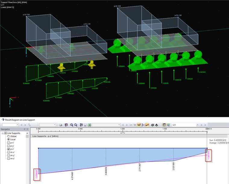
Note: The examples shown in this article have been calculated with a rough FE mesh so that the procedure can be illustrated with examples. With the "Result Diagrams" option from the shortcut menu of the line support, only the linear diagram with its ordinates at the support points (without the information in the info window) is transferred to the opened dialog box. Therefore, the linear smoothing in the dialog box shows a slightly different linear smoothing than directly in the work window. If the FE mesh size is reduced ever further so that the polygonal distribution adapts increasingly to a curved distribution, smaller and smaller errors are made when integrating the surface and determining the centroid.