
In RFEM and RSTAB, you can visualize the flow field quantities of pressure, velocity, turbulence kinetic energy, and turbulence dissipation rate for the wind simulation.
The clipping planes are aligned with the respective wind direction.
.png?mw=640&hash=9de889f94dda719e52d438f3fb6a495d2dce9a98)
Use the "Independent mesh preferred" option in the FE mesh settings to create an independent FE mesh for the integrated objects.
This allows you to generate a significantly more detailed and precise FE mesh for individual objects that are integrated into one another.
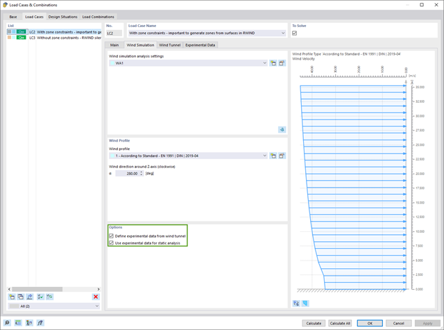
If you have experimentally determined surface pressures available for a model, you can apply them to a structural model in RFEM 6, process them in RWIND 2, and use them as wind loads in the structural analysis of RFEM 6.
You can find out how to apply the experimentally determined values in this technical article.
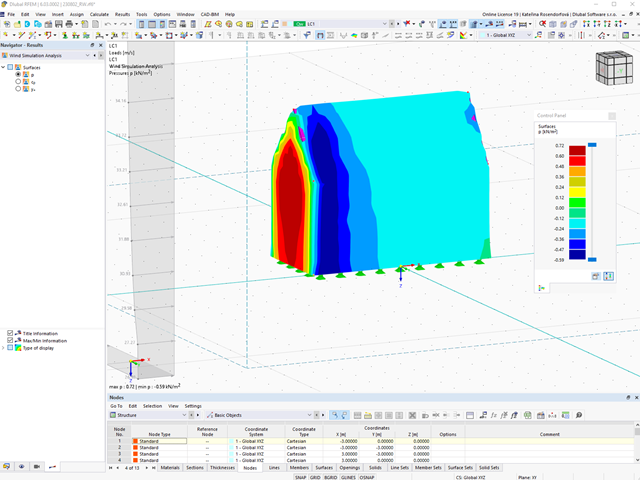
You can display the RWIND results directly in the main program. In the Navigator - Results, select the Wind Simulation Analysis result type from the list above.
Currently, the following results are available, which refer to the RWIND computational mesh:
- Surface pressure
- Surface cp coefficient
- Wall distance y+ (steady flow)
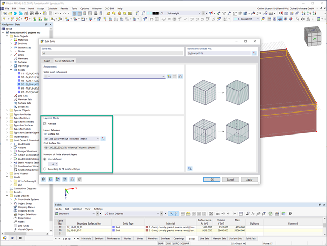
For the meshing of solids, you have the option of arranging a layered FE mesh. This option allows you to perform a defined division of the solid with finite elements between two parallel surfaces.
Go to Explanatory Video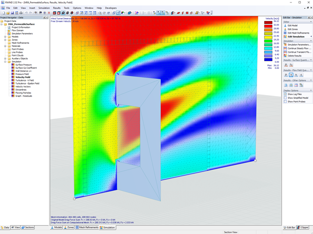
Use RWIND 2 Pro to easily apply a permeability to a surface. All you need is the definition of
- the Darcy coefficient D,
- the inertial coefficient I, and
- the length of the porous medium in the direction of flow L,
to define a pressure boundary condition between the front and back of a porous zone. Due to this setting, you obtain the flow through this zone with a two-part result display on both sides of the zone area.
But that's not all. Furthermore, the generation of a simplified model recognizes permeable zones and takes into account the corresponding openings in the model coating. Can you waive an elaborate geometric modeling of the porous element? Understandable – we have good news for you then! With a pure definition of the permeability parameters, you can avoid complex geometric modeling of the porous element. Use this feature to simulate permeable scaffolding, dust curtains, mesh structures, and so on.
More Information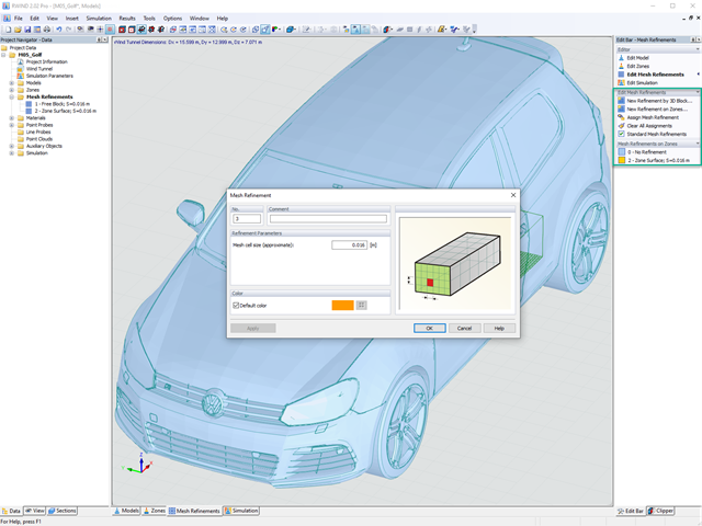
Do you already know the editor for mesh refinement control? It is a great help for your work! Why? It's easy – it gives you the following options:
- Graphic visualization of the areas with mesh refinements
- Mesh refinement of zones
- Deactivating the standard 3D solid mesh refinement with transversion into the corresponding manual 3D mesh refinements.
These options help you to formulate a suitable rule for meshing the entire model, even for the models with unusual dimensions. Use the editor to efficiently define small model details on large buildings or detailed meshing areas in the coating area of the model. You will be amazed!

The soil solids that you want to analyze are summarized in soil massifs.
Use the soil samples as a basis for a definition of the respective soil massif. This way, the program allows for user-friendly generation of the massif, including the automatic determination of the layer interfaces from the sample data, as well as the groundwater level and the boundary surface supports.
Soil massifs provide you with the option to specify a target FE mesh size independently of the global setting for the rest of the structure. You can thus consider the various requirements of the building and soil in the entire model.

Have you already discovered the tabular and graphical output of masses in mesh points? That's right, this is also part of the modal analysis results in RFEM 6. This way, you can check the imported masses that depend on various settings of the modal analysis. They can be displayed in the Masses in Mesh Points tab of the Results table. The table provides you with an overview of the following results: Mass - Translational Direction (mX, mY, mZ), Mass - Rotational Direction (mφX, mφY, mφZ), and the Sum of Masses. Would it be best for you to have a graphical evaluation as quickly as possible? Then you can also graphically display the masses in mesh points.
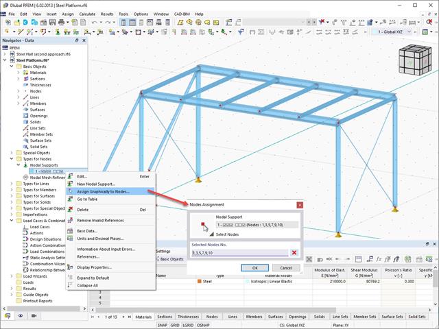
The object types listed below can be graphically assigned to the elements of the structure modeled in the program.
- Nodal supports
- Member shear panels
- Local reductions of member cross-sections
- Member transverse stiffeners
- Member longitudinal welds
- Effective lengths
- Boundary conditions
- Line supports
- Loads
- Member support
- Punching reinforcements
- Mesh refinements
- Surface reinforcements
- Surface results adjustments
- Surface support
- Service classes
- Imperfections
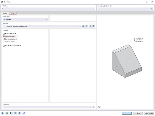
In addition to the "Mesh Refinement" and "Specific Direction" options for solids, you can also activate the "Grid for Results" option, which allows for organizing grid points in the solid space. Among other things, the center of gravity can be set as the origin. There is also the option to activate or deactivate the visibility of the grid for numerical results in "Navigator – Display" under Basic Objects.
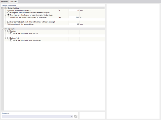
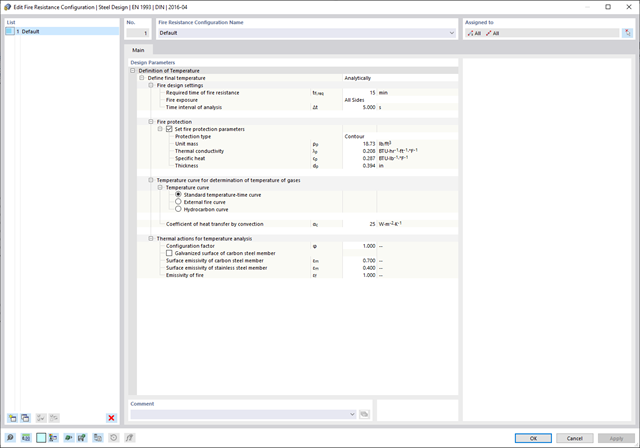
RFEM/RSTAB also provides a range of functions for the case of a fire. The program allows for the automatic generation of load and result combinations for the accidental design situation of fire design. The members to be designed with the corresponding internal forces are imported directly from RFEM/RSTAB. Also, all information about the material and cross-section is stored. You don't need to do anything else.
You only define the parameters relevant for the fire resistance design by assigning a fire resistance configuration to the members and surfaces to be designed. Moreover, you can also make further detailed settings, such as the definition of the fire exposure on one side up to all sides.
The structural analysis programs RFEM/RSTAB offer you a wide range of automated functions that make your dayily work easier. One of them is the automatic generation of load and result combinations for the accidental design situation of fire design. The members to be designed with the corresponding internal forces are imported directly from RFEM/RSTAB. You don't need to do anything else. The program has also already stored all information about the material and cross-section for you.
By assigning a fire resistance configuration to the members to be designed, you define the parameters relevant for the fire resistance design. Here you can manually specify the critical steel temperature at the design time. Or let the program to determine the temperature determined automatically for a specified fire duration. You can select from various fire temperature curves and fire protection measures. It is also possible to make further detailed settings, such as the definition of the fire exposure on all sides or three sides
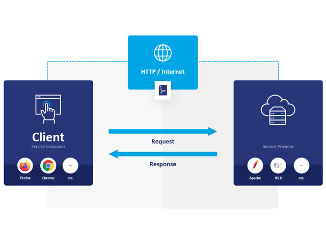
WebService and API provide you various scope of application. We have summarized some ideas as to how WebService and API can support your company:
- Creating additional applications for RFEM 6, RSTAB 9, and RSECTION 1
- Possibility to make the workflows more efficient (for example, model definition and input) and to integrate RFEM 6, RSTAB 9, and RSECTION 1 into your company applications
- Simulating and calculating several design options
- Running optimization algorithms for size, shape, and/or topology
- Accessing the calculation results
- Generation of printout reports in the PDF format
The level of quality of the work is automatically increased not only by the algorithmic model definitions, but also by:
- Extending / consolidating RFEM 6, RSTAB 9, and RSECTION 1 with your own controls
- Increased interoperability between the individual software used to complete a project
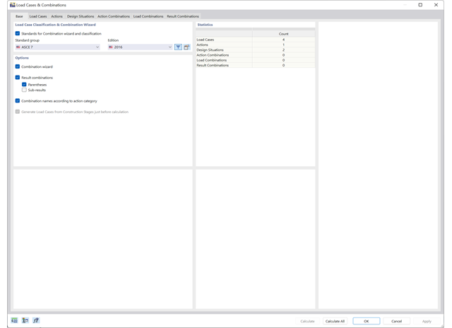
Use the new combination wizards to make your work easier. They fill the design situations with load or result combinations on the basis of an automatic or semi-automatic generation conforming to the standards.
RFEM is entering a new phase with RFEM 6! The new generation of the 3D FEA software is also used for the structural analysis of members, surfaces, and solids. Many of the tried and tested features remain, but we have improved them and added new features to make your work with RFEM even easier.
What particularly distinguishes RFEM 6 is the modern design concept, with the add-ons integrated directly into the program. Curious to learn more?

- Calculation of stationary incompressible turbulent wind flow using the SimpleFOAM solver from the OpenFOAM® software package
- Numerical scheme according to the first and second order
- Turbulence models RAS k-ω and RAS k-ε
- Consideration of surface roughness depending on model zones
- Model design via VTP, STL, OBJ, and IFC files
- Operation via bidirectional interface of RFEM or RSTAB for importing model geometries with standard-based wind loads and exporting wind load cases with probe-based printout report tables
- Intuitive model changes via drag & drop and graphical adjustment assistance
- Generation of a shrink-wrap mesh envelope around the model geometry
- Consideration of environmental objects (buildings, terrain, and so on)
- Height-dependent description of the wind load (wind speed and turbulence intensity)
- Automatic meshing depending on a selected depth of detail
- Consideration of layer meshes near the model surfaces
- Parallelized calculation with optimal utilization of all processor cores of a computer
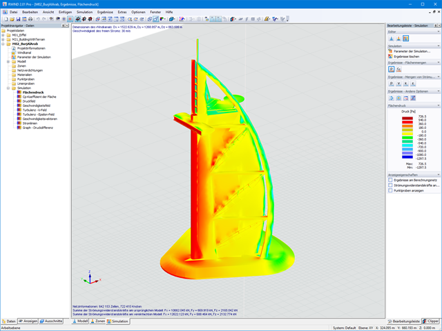
- Graphical output of the surface results on the model surfaces (surface pressure, Cp coefficients)
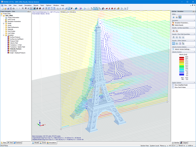
- Graphical output of the flow field and vector results (pressure field, velocity field, turbulence – k-ω field, and turbulence – k-ε field, velocity vectors) on Clipper/Slicer planes
- Display of 3D wind flow via animated streamline graphics
- Definition of point and line probes
- Multilingual user interface (German, English, Czech, Spanish, French, Italian, Polish, Portuguese, Russian, and Chinese)
- Calculations of several models in one batch process
- Generator for creating rotated models to simulate different wind directions
- Optional interruption and continuation of the calculation
- Individual color panel per result graphic
- Display of diagrams with separate output of results on both sides of a surface
- Output of the dimensionless wall distance y+ in the mesh inspector details for the simplified model mesh
- Determination of the shear stress on the model surface from the flow around the model
- Calculation with an alternative convergence criterion (you can select between the residual types pressure or flow resistance in the simulation parameters)
- Calculation of transient incompressible turbulent wind flow with the BlueDyMSolver solver
- LES SpalartAllmarasDDES turbulence model
- Consideration of stationary solution as initial state for transient calculation
- Automatic determination of analysis period and time steps
- Use of intermediate results during the calculation
- Organized display of time-varying results via time step units
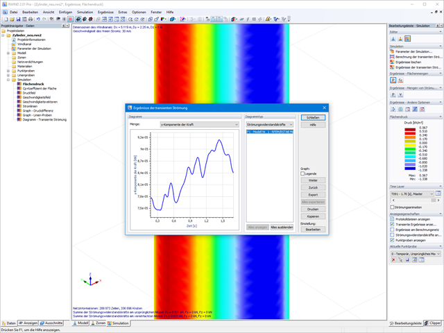
- Diagram of drag force and point probe results over analysis time
- Display of line probe results for any time steps in a diagram
- Freely adjustable wind permeability for surfaces (Go to Product Feature)
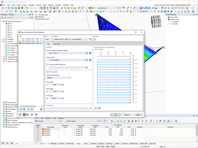
To model structures in RWIND Basic, you find a special application in RFEM and RSTAB. Here, you define the wind directions to be analyzed by means of related angular positions about the vertical model axis. At the same time, you define the elevation-dependent wind profile on the basis of a wind standard. In addition to these specifications, you can use the stored calculation parameters to determine your own load cases for a stationary calculation per each angular position.
As an alternative, you can also use the RWIND Basic program manually, without the interface application in RFEM or RSTAB. In this case, RWIND Basic models the structures and terrain environment directly from the imported VTP, STL, OBJ, and IFC files. You can define the height-dependent wind load and other fluid-mechanical data directly in RWIND Basic.
RWIND Basic uses a numerical CFD model (Computational Fluid Dynamics) to simulate wind flows around your objects using a digital wind tunnel. The simulation process determines specific wind loads acting on your model surfaces from the flow result around the model.
A 3D volume mesh is responsible for the simulation itself. For this, RWIND Basic performs an automatic meshing on the basis of freely definable control parameters. For the calculation of wind flows, RWIND Basic provides you with a stationary solve and RWIND Pro provides a transient solver for incompressible turbulent flows. Surface pressures resulting from the flow results are extrapolated onto the model for each time step.
By solving the numerical flow problem, you can obtain the following results on and around the model:
- Pressure on structure surface
- Coefficient Cp distribution on the structure surfaces
- Pressure field about the structure geometry
- Velocity field about the structure geometry
- Turbulence k-ω field about the structure geometry
- Turbulence k-ε field about the structure geometry
- Velocity vectors about the structure geometry
- Streamlines about the structure geometry
- Forces on member-shaped structures that were originally generated from member elements
- Convergence diagram
- Direction and size of the flow resistance of the defined structures
Despite this amount of information, RWIND 2 remains clearly arranged, as is typical for the Dlubal programs. You can specify freely definable zones for a graphic evaluation. Voluminously displayed flow results about the structure geometry are often confusing – you know the problem for sure. That's why RWIND Basic provides freely movable section planes for the separate display of the "solid results" in a plane. For the 3D branched streamline result, you have an option to select between a static and an animated display in the form of moving line segments or particles. This option helps you to represent the wind flow as a dynamic effect.
You can export all results as a picture or, especially for the animated results, as a video.
When starting the analysis in the RFEM or RSTAB application, you trigger a batch process. It places all member, surface, and solid definitions of the model rotated with all relevant coefficients in the numerical wind tunnel of RWIND Basic. Furthermore, it starts the CFD analysis, and returns the resulting surface pressures for a selected time step as FE mesh nodal loads or member loads into the respective load cases of RFEM or RSTAB.
These load cases which contain RWIND Basic loads can then be calculated. Moreover, you can combine them with other loads in load and result combinations.
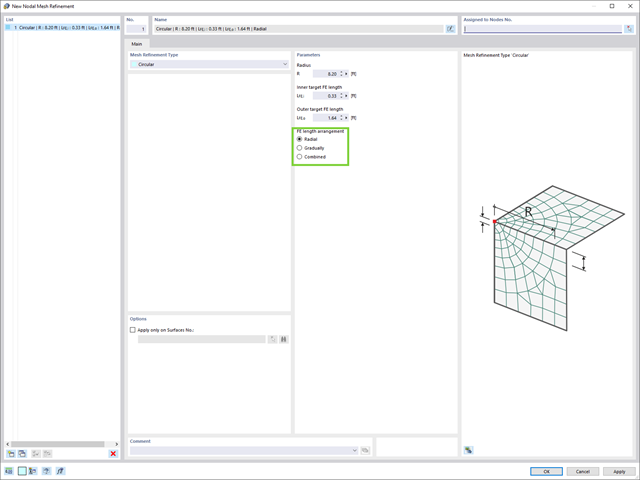
There's something new for you! To define odal mesh refinements, the options for FE length arrangement have been added:
- Radial
- Gradually
- Combined

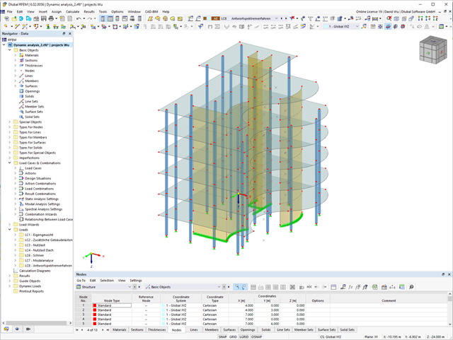
Compared to the RF‑/DYNAM Pro - Natural Vibrations add-on module (RFEM 5 / RSTAB 8), the following new features have been added to the Modal Analysis add-on for RFEM 6 / RSTAB 9:
- Preset combination coefficients for various standards (EC 8, ASCE, and so on)
- Optional neglect of masses (for example, mass of foundations)
- Methods for determining the number of mode shapes (user-defined, automatic - to reach effective modal mass factors, automatic - to reach the maximum natural frequency)
- Output of modal masses, effective modal masses, modal mass factors, and participation factors
- Masses in mesh points displayed in tables and graphics
- Various scaling options for mode shapes in the Result navigator

Do you know exactly how the form-finding is performed? First, the form-finding process of the load cases with the load case category "Prestress" shifts the initial mesh geometry to an optimally balanced position by means of iterative calculation loops. For this task, the program uses the Updated Reference Strategy (URS) method by Prof. Bletzinger and Prof. Ramm. This technology is characterized by equilibrium shapes that, after the calculation, comply almost exactly with the initially specified form-finding boundary conditions (sag, force, and prestress).
In addition to the pure description of the expected forces or sags on the elements to be formed, the integral approach of the URS also enables a consideration of regular forces. In the overall process, this allows, for example, for a description of the self-weight or a pneumatic pressure by means of corresponding element loads.
All these options give the calculation kernel the potential to calculate anticlastic and synclastic forms that are in an equilibrium of forces for planar or rotationally symmetric geometries. In order to be able to realistically implement both types individually or together in one environment, the calculation provide you with two ways to describe the form-finding force vectors:
- Tension method - description of the form-finding force vectors in space for planar geometries
- Projection method - description of the form-finding force vectors on a projection plane with fixation of the horizontal position for conical geometries

Was your design successful? Then just sit back and relax. You benefit from the numerous functions in RFEM also here. The program gives you the maximum stresses of the masonry surfaces, whereby you can display the results in detail at each FE mesh point.
Moreover, you can insert sections in order to carry out a detailed evaluation of the individual areas. Use the display of the yield areas to estimate the cracks in the masonry.
_(1).png?mw=640&hash=415f7bbaf70e41679bb0106e1cf91eaa8c493ec9)
- Automatic generation of FE analysis models: The add-on automatically creates a finite element model (FE) of the steel connection in the background.
- Consideration of all internal forces: The calculation and design checks include all internal forces (N, Vy, Vz, My, Mz, MT) and are not limited to planar loading.
- Automatic load transfer: All load combinations are automatically transferred to the FE analysis model of the connection. The loads are transferred directly from RFEM, so manual data input is not necessary.
- Efficient modeling: The add-on saves you time when modeling complex connection situations. You can also save the created FE analysis model and use it further for your own detailed analyses.
- Extensible library: An extensive and extensible library with predefined steel connection templates is available.
- Wide applicability: The add-on is suitable for connections of any type and shape, compatible with almost all rolled, welded, built-up, and thin-walled cross-sections.

- Automatic consideration of masses from self-weight
- Direct import of masses from load cases or load combinations
- Optional definition of additional masses (nodal, linear, or surface masses, as well as inertia masses) directly in the load cases
- Optional neglect of masses (for example, mass of foundations)
- Combination of masses in different load cases and load combinations
- Preset combination coefficients for various standards (EC 8, SIA 261, ASCE 7,...)
- Optional import of initial states (for example, to consider prestress and imperfection)
- Structure Modification
- Consideration of failed supports or members/surfaces/solids
- Definition of several modal analyses (for example, to analyze different masses or stiffness modifications)
- Selection of mass matrix type (diagonal matrix, consistent matrix, unit matrix), including user-defined specification of translational and rotational degrees of freedom
- Methods for determining the number of mode shapes (user-defined, automatic - to reach effective modal mass factors, automatic - to reach the maximum natural frequency - only available in RSTAB)
- Determination of mode shapes and masses in nodes or FE mesh points
- Results of eigenvalue, angular frequency, natural frequency, and period
- Output of modal masses, effective modal masses, modal mass factors, and participation factors
- Masses in mesh points displayed in tables and graphics
- Visualization and animation of mode shapes
- Various scaling options for mode shapes
- Documentation of numerical and graphical results in printout report
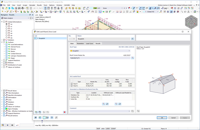
Do you want your structures to remain upright even in wind and snow? Then rely on the load wizards for plate and frame structures. You can now generate wind loads according to EN 1991‑1‑4 and snow loads according to EN 1991‑1‑3 (as well as other international standards). The load cases are generated depending on the roof shape.
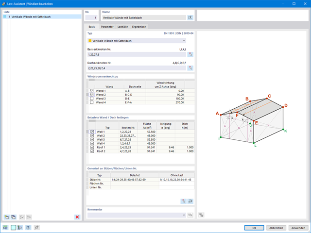
Wind loads are also not a problem in your design. You can automatically generate wind loads as member loads or area loads (RFEM) on the following structural components:
- Vertical walls
- Flat roofs
- Monopitch roofs
- Duopitch/troughed roofs
- Vertical walls with duopitch roof
- Vertical walls with flat/monopitch roof
The following standards are available to you:
-
 EN 1991-1-4 (including National Annexes)
 -
 ASCE 7
 -
 CTE DB-SE-AE
 -
 GB 50009