SHAPE-THIN determines the section properties and stresses of any open, closed, built-up, or non-connected cross-sections.
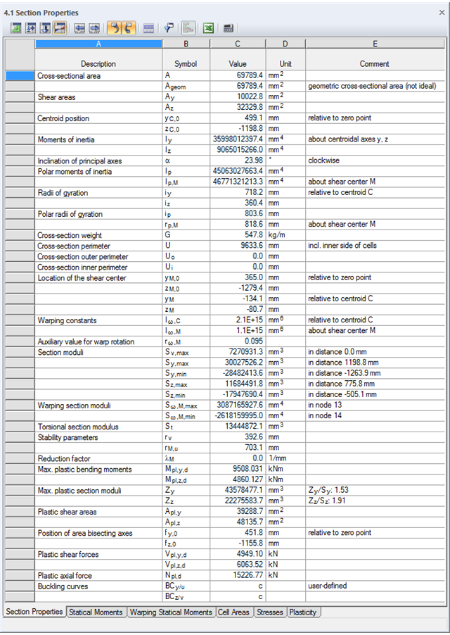
- Section Properties
- Cross-sectional area A
- Shear areas Ay, Az, Au, and Av
- Centroid position yS, zS
- moments of area 2 degrees Iy, Iz, Iyz, Iu, Iv, Ip, Ip,M
- Radii of gyration iy, iz, iyz, iu, iv, ip, ip,M
- Inclination of principal axes α
- Cross-section weight G
- Cross-section perimeter U
- torsional constants of area degrees IT, IT,St.Venant, IT,Bredt, IT,s
- Location of the shear center yM, zM
- Warping constants Iω,S, Iω,M or Iω,D for lateral restraint
- Max/min section moduli Sy, Sz, Su, Sv, Sω,M with locations
- Section ranges ru, rv, rM,u, rM,v
- Reduction factor λM
- Plastic Cross-Section Properties
- Axial force Npl,d
- Shear forces Vpl,y,d, Vpl,z,d, Vpl,u,d, Vpl,v,d
- Bending moments Mpl,y,d, Mpl,z,d, Mpl,u,d, Mpl,v,d
- Section moduli Zy, Zz, Zu, Zv
- Shear areas Apl,y, Apl,z, Apl,u, Apl,v
- Position of area bisecting axes fu, fv,
- Display of the inertia ellipse
- First moments of area Qu, Qv, Qy, Qz with location of maxima and specification of shear flow
- Warping coordinates ωM
- moments of area (warping areas) Sω,M
- Cell areas Am of closed cross-sections
- Normal stresses σx due to axial force, bending moments, and warping bimoment
- Shear stresses τ from shear forces as well as primary and secondary torsional moments
- Equivalent stresses σv with customizable factor for shear stresses
- Stress ratios, related to limit stresses
- Stresses for element edges or center lines
- Weld stresses in fillet welds
- Section properties of non-connected cross-sections (cores of high-rise buildings, composite sections)
- Shear wall shear forces due to bending and torsion
- Plastic capacity design with determination of the enlargement factor αpl
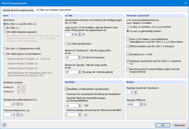
- Check of the c/t-ratios following the design methods el-el, el-pl or pl-pl according to DIN 18800
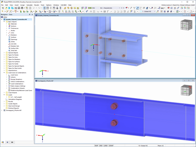
In the Steel Joint add-on, you can design the connections of members with composite cross-sections. Furthermore, you can perform joint design checks for almost all thin-walled cross-sections in the RFEM library.
Go to Explanatory Video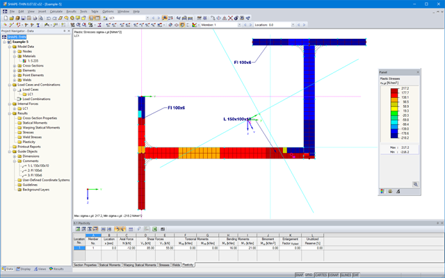
All results can be evaluated and visualized in an appealing numerical and graphical form. Selection functions facilitate the targeted evaluation.
The printout report corresponds to the high standards of RFEM and rstab/rstab-9/what-is-rstab RSTAB. Modifications are updated automatically.

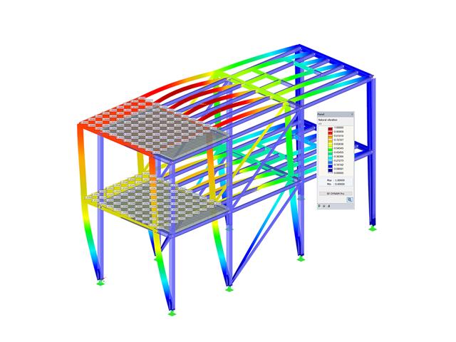
As you've already learned, the results of a Modal Analysis load case are displayed in the program after a successful calculation. You can thus immediately see the first mode shape graphically or as an animation. You can also easily adjust the representation of the mode shape standardization. Do that directly in the Results navigator, where you have one of four options for the visualization of the mode shapes available for the selection:
- Scaling the value of the mode shape vector uj to 1 (considers the translation components only)
- Selecting the maximum translational component of the eigenvector and setting it to 1
- Considering the entire eigenvector (including the rotation components), selecting the maximum, and setting it to 1
- Setting the modal mass mi for each mode shape to 1 kg
You can find a detailed explanation of the mode shape standardization in the OnlineManual here.
SHAPE-THIN calculates all relevant cross‑section properties, including plastic limit internal forces. Overlapping areas are set close to reality. If cross-sections consist of different materials, SHAPE‑THIN determines the effective cross‑section properties with respect to the reference material.
In addition to the elastic stress analysis, you can perform the plastic design including interaction of internal forces for any cross‑section shape. The plastic interaction design is carried out according to the Simplex Method. You can select the yield hypothesis according to Tresca or von Mises.
SHAPE-THIN performs a cross-section classification according to EN 1993-1-1 and EN 1999-1-1. For steel cross-sections of cross-section class 4, the program determines effective widths for unstiffened or stiffened buckling panels according to EN 1993-1-1 and EN 1993-1-5. For aluminum cross-sections of cross-section class 4, the program calculates effective thicknesses according to EN 1999-1-1.
Optionally, SHAPE‑THIN checks the limit c/t-values in compliance with the design methods el‑el, el‑pl, or pl‑pl according to DIN 18800. The c/t-zones of elements connected in the same direction are recognized automatically.

Is the calculation finished? The results of the modal analysis are then available both graphically and in tables. Display the result tables for the load case or the load cases of the modal analysis. Thus, you can see the eigenvalues, angular frequencies, natural frequencies, and natural periods of the structure at first glance. The effective modal masses, modal mass factors, and participation factors are also clearly displayed.
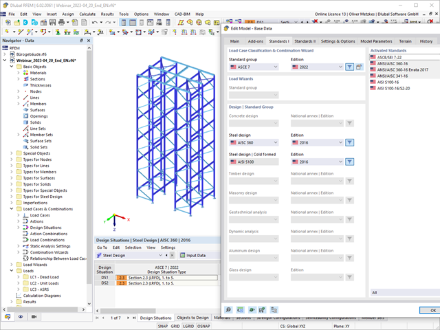
The design of cold-formed steel members according to the AISI S100-16 / CSA S136-16 is available in RFEM 6. Design can be accessed by selecting “AISC 360” or “CSA S16” as the standard in the Steel Design Add-on. “AISI S100” or “CSA S136” is then automatically selected for the cold-formed design.
RFEM applies the Direct Strength Method (DSM) to calculate the elastic buckling load of the member. The Direct Strength Method offers two types of solutions, numerical (Finite Strip Method) and analytical (Specification). The FSM signature curve and buckling shapes can be viewed under Sections.
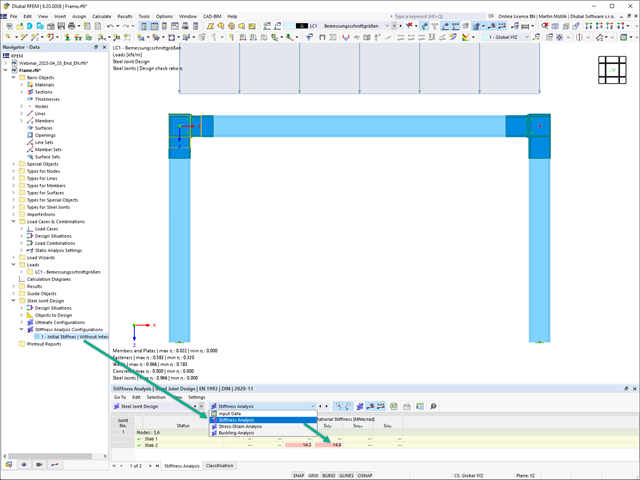
The initial stiffness Sj,ini is a crucial parameter for evaluating whether a connection can be characterized as rigid, semi-rigid, or pinned.
In the "Steel Joints" add-on, you can calculate the initial stiffness Sj,ini according to Eurocode (EN 1993‑1‑8, Section 5.2.2) and AISC (AISC 360-16, Cl. E3.4) with regard to the internal forces N, My, and/or Mz.
The optional automatic transfer of initial stiffnesses allows for a directly transfer as member hinge stiffnesses in RFEM. The entire structure is then recalculated and the resulting internal forces are automatically adopted as loads in the analysis and design of the connection models.
This automated iteration process eliminates the need for manual export and import of data, reducing the amount of work and minimizing potential sources of error.
Explanatory Video: Calculation of Initial Stiffness Sj,ini
You can perform the calculation of the warping torsion on the entire system. Thus, you consider the additional 7th degree of freedom in the member calculation. The stiffnesses of the connected structural elements are automatically taken into account. It means, you don't need to define equivalent spring stiffnesses or support conditions for a detached system.
You can then use the internal forces from the calculation with warping torsion in the add-ons for the design. Consider the warping bimoment and the secondary torsional moment, depending on the material and the selected standard. A typical application is the stability analysis according to the second-order theory with imperfections in steel structures.
Did you know that The application is not limited to thin-walled steel cross-sections. Thus, it is possible for you, for example, to perform the calculation of the ideal overturning moment of beams with solid timber cross-sections.
- Response spectra in accordance with different standards
- The following standards are implemented:
-
 EN 1998-1:2010 + A1:2013 (European Union)
 -
 DIN 4149:1981-04 (Germany)
 -
DIN 4149:2005-04 (Germany)
-
 IBC 2000 (USA)
 -
IBC 2009-ASCE/SEI 7-05 (USA)
-
IBC 2012/15 - ASCE/SEI 7-10 (USA)
-
IBC 2018 - ASCE/SEI 7-16 (USA)
-
 ÖNORM B 4015:2007-02 (Austria)
 -
 NTC 2018 (Italy)
 -
 NCSE-02 (Spain)
 -
 SIA 261/1:2003 (Switzerland)
 -
SIA 261/1:2014 (Switzerland)
-
SIA 261/1: 2020 (Switzerland)
-
 O.G. 23089 + OG 23390 (Turkey)
 -
 SANS 10160-4 2010 (South Africa)
 -
 SBC 301:2007 (Saudi Arabia)
 -
 GB 50011 - 2001 (China)
 -
GB 50011 - 2010 (China)
-
 NBC 2015 (Canada)
 -
 DTR BC 2-48 (Algeria)
 -
DTR RPA99 (Algeria)
-
 CFE Sismo 08 (Mexico)
 -
 CIRSOC 103 (Argentina)
 -
 NSR - 10 (Colombia)
 -
 IS 1893:2002 (India)
 -
 AS1170.4 (Australia)
 -
 NCh 433 1996 (Chile)
-
- The following National Annexes according to EN 1998‑1 are available:
-
DIN EN 1998-1/NA:2011-01 (Germany)
-
ÖNORM EN 1991-1-1:2011-09 (Austria)
-
 NBN - ENV 1998-1-1: 2002 NAD-E/N/F (Belgium)
 -
 ČSN EN 1998-1/NA:2007 (Czech Republic)
 -
 NF EN 1998-1-1/NA:2014-09 (France)
 -
UNI-EN 1991-1-1/NA:2007 (Italy)
-
 NP EN 1998-1/NA:2009 (Portugal)
 -
 SR EN 1998-1/NA:2004 (Romania)
 -
 STN EN 1998-1/NA:2008 (Slovakia)
 -
 SIST EN 1998-1:2005/A101:2006 (Slovenia)
 -
 CYS EN 1998-1/NA:2004 (Cyprus)
 -
 NA to BS EN 1998-1:2004:2008 (United Kingdom)
 - NS-EN 1998-1:2004 + A1:2013/NA:2014 (Norway)
-
- User-defined response spectra
- Direction-relative response spectrum approach
- Relevant mode shapes for the response spectrum can be selected manually or automatically (5% rule from EC 8 can be applied)
- Generated equivalent static loads are exported to load cases, separately for each modal contribution and separately for each direction
- Result combinations by modal superposition (SRSS and CQC rule) and direction superposition (SRSS or 100% / 30% rule)
- Signed results based on the dominant eigenmode can be displayed