
If there is a load case or load combination in the program, the stability calculation is activated. You can define another load case in order to consider initial prestress, for example.
For this, you need to specify whether to perform a linear or nonlinear analysis. Depending on the case of application, you can select a direct calculation method, such as the Lanczos method or the ICG iteration method. Members not integrated in surfaces are usually displayed as member elements with two FE nodes. With such elements, the program cannot determine the local buckling of single members. That's why you have the option to divide members automatically.

You can select several methods that are available for the eigenvalue analysis:
- Direct Methods
- The direct methods (Lanczos [RFEM], roots of characteristic polynomial [RFEM], subspace iteration method [RFEM/RSTAB], and shifted inverse iteration [RSTAB]) are suitable for small to medium-sized models. You should only use these fast solver methods if your computer has a larger amount of memory (RAM).
- ICG Iteration Method (Incomplete Conjugate Gradient [RFEM])
- In contrast, this method only requires a small amount of memory. Eigenvalues are determined one after the other. It can be used to calculate large structural systems with few eigenvalues.
Use the Structure Stability add-on to perform a nonlinear stability analysis using the incremental method. This analysis delivers close-to-reality results also for nonlinear structures. The critical load factor is determined by gradually increasing the loads of the underlying load case until the instability is reached. The load increment takes into account nonlinearities such as failing members, supports and foundations, and material nonlinearities. After increasing the load, you can optionally perform a linear stability analysis on the last stable state in order to determine the stability mode.

As the first results, the program presents you with the critical load factors. You can then perform an evaluation of stability risks. For member models, the resulting effective lengths and critical loads of the members are displayed to you in tables.
Use the next result window to check the normalized eigenvalues sorted by node, member, and surface. The eigenvalue graphic allows you to evaluate the buckling behavior. This makes it easier for you to take countermeasures.

- Calculation of models consisting of member, shell, and solid elements
- Nonlinear stability analysis
- Optional consideration of axial forces from initial prestress
- Four equation solvers for an efficient calculation of various structural models
- Optional consideration of stiffness modifications in RFEM/RSTAB
- Determination of a stability mode greater than the user-defined load increment factor (Shift method)
- Optional determination of the mode shapes of unstable models (to identify the cause of instability)
- Visualization of the stability mode
- Basis for determining imperfection
- Consideration of 7 local deformation directions (ux, uy, uz, φx, φy, φz, ω) or 8 internal forces (N, Vu, Vv, Mt,pri, Mt,sec, Mu, Mv, Mω) when calculating member elements
- Usable in combination with a structural analysis according to linear static, second-order, and large deformation analysis (imperfections can also be taken into account)
- In combination with the Stability Analysis add-on, allows you to determine critical load factors and mode shapes of stability problems such as torsional buckling and lateral-torsional buckling
- Consideration of end plates and transverse stiffeners as warping springs when calculating I-sections with automatic determination and graphical display of the warping spring stiffness
- Graphical display of the cross-section warping of members in the deformation
- Full integration with RFEM and RSTAB

You can perform the calculation of the warping torsion on the entire system. Thus, you consider the additional 7th degree of freedom in the member calculation. The stiffnesses of the connected structural elements are automatically taken into account. It means, you don't need to define equivalent spring stiffnesses or support conditions for a detached system.
You can then use the internal forces from the calculation with warping torsion in the add-ons for the design. Consider the warping bimoment and the secondary torsional moment, depending on the material and the selected standard. A typical application is the stability analysis according to the second-order theory with imperfections in steel structures.
Did you know that The application is not limited to thin-walled steel cross-sections. Thus, it is possible for you, for example, to perform the calculation of the ideal overturning moment of beams with solid timber cross-sections.

- You can activate or deactivate the use of torsional warping in the Add-ons tab of the model's Base Data.
- After activating the add-on, the user interface in RFEM is extended by some new entries in the navigator, tables, and dialog boxes.

- Realistic representation of interaction between a building and soil
- Realistic representation of the influences of the foundation components on each other
- Extensible library of soil properties
- Consideration of several soil samples (probes) at different locations, even outside the building
- Determination of settlements and stress diagrams as well as their graphical and tabular display

Entering soil layers for soil samples is performed in a clearly arranged dialog box. A corresponding graphical representation supports clarity and makes checking the input user-friendly.
An extensible database facilitates the selection of soil material properties. The Mohr-Coulomb model as well as a nonlinear model with stress and strain dependent stiffness are available for a realistic modeling of the soil material behavior.
You can define any number of soil samples and layers. The soil is generated from all entered samples using 3D solids. Assignment to the structure is carried out using coordinates.
The soil body is calculated according to the nonlinear iterative method. The calculated stresses and settlements are displayed graphically and in tables.
- Simple definition of construction stages in the RFEM structure including visualization
- Adding, removing, modifying, and reactivating member, surface, and solid elements and their properties (for example, member and line hinges, degrees of freedom for supports, and so on)
- Automatic and manual combinatorics with load combinations in the individual construction stages (for example, to consider mounting loads, mounting cranes, and other loads)
- Consideration of nonlinear effects such as tension member failure or nonlinear supports
- Interaction with other add-ons, such as Nonlinear Material Behavior, Structure Stability, Form-Firnding, and so on.
- Display of results numerically and graphically for individual construction stages
- Detailed printout report with documentation of all structural and load data for each construction stage

Have you created the entire structure in RFEM? Very well, now you can assign the individual structural components and load cases to the corresponding construction stages. In each construction stage, you can modify release definitions of members and supports, for example.
You can thus model structural modifications, such as those that occur when bridge girders are successively grouted or when columns are settled. Then, assign the load cases created in RFEM to the construction stages as permanent or non-permanent loads.
Did you know that The combinatorics allows you to superimpose the permanent and non-permanent loads in load combinations. In this way, it is possible for you to determine the maximum internal forces of different crane positions or to consider temporary mounting loads available in one construction stage only.

If there are geometry differences arising between the ideal and the deformed structural system from the previous construction stage, they are compared in the program. The next construction stage is built on top of the stressed system from the previous construction stage. This calculation is nonlinear.

Was the calculation successful? Now you can view the results of the individual construction stages graphically and in tables in RFEM. Moreover, RFEM allows you to consider the construction stages in the combinatorics and include it in further design.

The Dlubal structural analysis software does a lot of work for you. The input parameters, which are relevant for the selected standards, are suggested by the program in accordance with the rules. Furthermore, you can enter response spectra manually.
Load cases of the type Response Spectrum Analysis define the direction in which response spectra act and which eigenvalues of the structure are relevant for the analysis. In the spectral analysis settings, you can define details for the combination rules, damping (if applicable), and zero-period acceleration (ZPA).

Did you know that Equivalent static loads are generated separately for each relevant eigenvalue and excitation direction. These loads are saved in a load case of the Response Spectrum Analysis type and RFEM/RSTAB performs a linear static analysis.

The load cases of the type Response Spectrum Analysis contain the generated equivalent loads. First, the modal contributions have to be superimposed with the SRSS or CQC rule. In this case, you can use the signed results based on the dominant mode shape.
Afterwards, the directional components of earthquake actions are combined with the SRSS or the 100% / 30% rule.

- Stress determination using an elastic-plastic material model
- Design of masonry disc structures for compression and shear on the building model or single model
- Automatic determination of stiffness of a wall-slab hinge
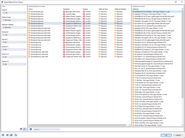
- An extensive material database for almost all stone-mortar combinations available on the Austrian market (the product range is continuously being expanded, for other countries as well)
- Automatic determination of material values according to Eurocode 6 (ÖN EN 1996‑X)
- Option to create pushover analysis
You enter and model the structure directly in RFEM. You can combine the masonry material model with all common RFEM add-ons. This enables you to design the entire building models in connection with masonry.
The program automatically determines for you all parameters required for the calculation by using the material data that you have entered. Then, it finally generates the stress-strain curves for each FE element.

Was your design successful? Then just sit back and relax. You benefit from the numerous functions in RFEM also here. The program gives you the maximum stresses of the masonry surfaces, whereby you can display the results in detail at each FE mesh point.
Moreover, you can insert sections in order to carry out a detailed evaluation of the individual areas. Use the display of the yield areas to estimate the cracks in the masonry.
Compared to the RF‑/STABILITY (RFEM 5) and RSBUCK (RSTAB 8) add-on modules, the following new features have been added to the Structure Stability add-on for RFEM 6 / RSTAB 9:
- Activation as a property of a load case or a load combination
- Automated activation of the stability calculation via combination wizards for several load situations in one step
- Incremental load increase with user-defined termination criteria
- Modification of the mode shape normalization without recalculation
- Result tables with filter option