
In the Geotechnical Analysis add-on, the Hoek-Brown material model is available. The model shows linear-elastic ideal-plastic material behavior. Its nonlinear strength criterion is the most common failure criterion for stone and rocks.
You can enter the material parameters using
- Rock parameters directly, or alternatively via
- GSI classification.
Detailed information about this material model and the definition of the input in RFEM can be found in the respective chapter Hoek-Brown Model of the online manual for the Geotechnical Analysis add-on.
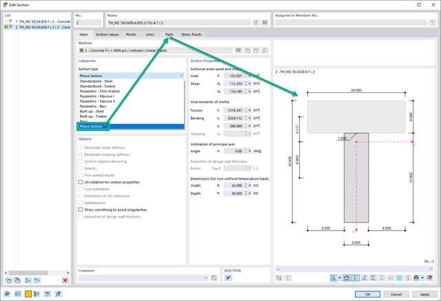
In the Construction Stages Analysis (CSA) add-on, you can use built-up cross-sections by means of what are known as phase sections. This allows you to activate and deactivate the parts of the "Parametric - Massive II" section type throughout the construction stages.

Building stone on stone has a long tradition in construction. The Masonry Design add-on for RFEM allows you to design masonry using the finite element method. It was developed as part of the research project DDMaS - Digitizing the Design of Masonry Structures. Here, the material model represents the nonlinear behavior of the brick-mortar combination in the form of macro-modeling. Do you want to find out more?

- Realistic representation of interaction between a building and soil
- Realistic representation of the influences of the foundation components on each other
- Extensible library of soil properties
- Consideration of several soil samples (probes) at different locations, even outside the building
- Determination of settlements and stress diagrams as well as their graphical and tabular display

For a response spectrum analysis of building models, you can display the sensitivity coefficients for the horizontal directions by story.
These key figures allow you to interpret the sensitivity to stability effects.

Enter and model a soil solid directly in RFEM. You can combine the soil material models with all common RFEM add-ons.
This allows you to easily analyze the entire models with a complete representation of the soil-structure interaction.
All parameters required for the calculation are automatically determined from the material data that you have entered. The program then generates the stress-strain curves for each FE element.

Have you created the entire structure in RFEM? Very well, now you can assign the individual structural components and load cases to the corresponding construction stages. In each construction stage, you can modify release definitions of members and supports, for example.
You can thus model structural modifications, such as those that occur when bridge girders are successively grouted or when columns are settled. Then, assign the load cases created in RFEM to the construction stages as permanent or non-permanent loads.
Did you know that The combinatorics allows you to superimpose the permanent and non-permanent loads in load combinations. In this way, it is possible for you to determine the maximum internal forces of different crane positions or to consider temporary mounting loads available in one construction stage only.
- Simple definition of construction stages in the RFEM structure including visualization
- Adding, removing, modifying, and reactivating member, surface, and solid elements and their properties (for example, member and line hinges, degrees of freedom for supports, and so on)
- Automatic and manual combinatorics with load combinations in the individual construction stages (for example, to consider mounting loads, mounting cranes, and other loads)
- Consideration of nonlinear effects such as tension member failure or nonlinear supports
- Interaction with other add-ons, such as Nonlinear Material Behavior, Structure Stability, Form-Firnding, and so on.
- Display of results numerically and graphically for individual construction stages
- Detailed printout report with documentation of all structural and load data for each construction stage

If there are geometry differences arising between the ideal and the deformed structural system from the previous construction stage, they are compared in the program. The next construction stage is built on top of the stressed system from the previous construction stage. This calculation is nonlinear.
Compared to the RF‑/STAGES add-on module (RFEM 5), the following new features have been added to the Construction Stages Analysis (CSA) add-on for RFEM 6:
- Consideration of construction stages at RFEM level
- Integration of the construction stage analysis into the combinatorics in RFEM
- Additional structural elements, such as line hinges, are supported
- Analysis of alternative construction processes in a model
- Reactivation of elements

Was the calculation successful? Now you can view the results of the individual construction stages graphically and in tables in RFEM. Moreover, RFEM allows you to consider the construction stages in the combinatorics and include it in further design.

The modal relevance factor (MRF) can help you to assess to which extent specific elements participate in a specific mode shape. The calculation is based on the relative elastic deformation energy of each individual member.
The MRF can be used to distinguish between local and global mode shapes. If multiple individual members show significant MRF (for example, > 20%), the instability of the entire structure or a substructure is very likely. On the other hand, if the sum of all MRFs for an eigenmode is around 100%, a local stability phenomenon (for example, buckling of a single bar) can be expected.
Furthermore, the MRF can be used to determine critical loads and equivalent buckling lengths of certain members (for example, for stability design). Mode shapes for which a specific member has small MRF values (for example, < 20%) can be neglected in this context.
The MRF is displayed by mode shape in the result table under Stability Analysis → Results by Members → Effective Lengths and Critical Loads.

The Dlubal structural analysis software does a lot of work for you. The input parameters, which are relevant for the selected standards, are suggested by the program in accordance with the rules. Furthermore, you can enter response spectra manually.
Load cases of the type Response Spectrum Analysis define the direction in which response spectra act and which eigenvalues of the structure are relevant for the analysis. In the spectral analysis settings, you can define details for the combination rules, damping (if applicable), and zero-period acceleration (ZPA).

- Calculation of models consisting of member, shell, and solid elements
- Nonlinear stability analysis
- Optional consideration of axial forces from initial prestress
- Four equation solvers for an efficient calculation of various structural models
- Optional consideration of stiffness modifications in RFEM/RSTAB
- Determination of a stability mode greater than the user-defined load increment factor (Shift method)
- Optional determination of the mode shapes of unstable models (to identify the cause of instability)
- Visualization of the stability mode
- Basis for determining imperfection
You enter and model the structure directly in RFEM. You can combine the masonry material model with all common RFEM add-ons. This enables you to design the entire building models in connection with masonry.
The program automatically determines for you all parameters required for the calculation by using the material data that you have entered. Then, it finally generates the stress-strain curves for each FE element.

- Stress determination using an elastic-plastic material model
- Design of masonry disc structures for compression and shear on the building model or single model
- Automatic determination of stiffness of a wall-slab hinge
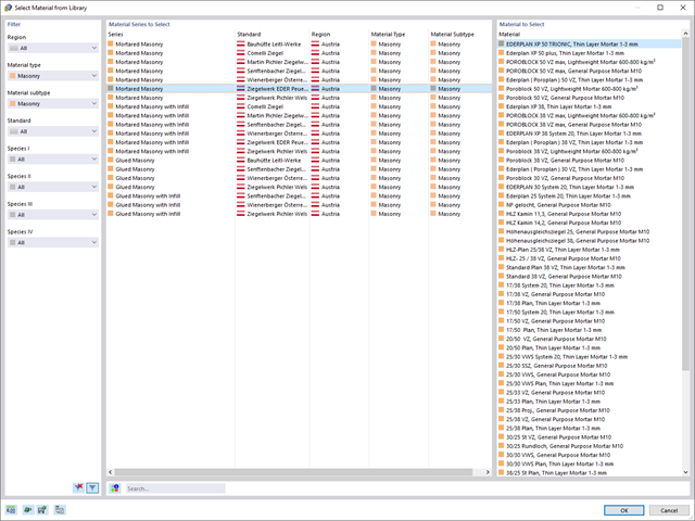
- An extensive material database for almost all stone-mortar combinations available on the Austrian market (the product range is continuously being expanded, for other countries as well)
- Automatic determination of material values according to Eurocode 6 (ÖN EN 1996‑X)
- Option to create pushover analysis

If there is a load case or load combination in the program, the stability calculation is activated. You can define another load case in order to consider initial prestress, for example.
For this, you need to specify whether to perform a linear or nonlinear analysis. Depending on the case of application, you can select a direct calculation method, such as the Lanczos method or the ICG iteration method. Members not integrated in surfaces are usually displayed as member elements with two FE nodes. With such elements, the program cannot determine the local buckling of single members. That's why you have the option to divide members automatically.

Compared to the RF-/DYNAM Pro - Equivalent Loads add-on module (RFEM 5 / RSTAB 8), the following new features have been added to the Response Spectrum Analysis add-on for RFEM 6 / RSTAB 9:
- Response spectra of numerous standards (EN 1998, DIN 4149, IBC 2018, and so on)
- User-defined response spectra or those generated from accelerograms
- Direction-relative response spectrum approach
- Results are stored centrally in a load case with underlying levels to ensure clarity
- Accidental torsional actions can be taken into account automatically
- Automatic combinations of seismic loads with the other load cases for use in an accidental design situation

Entering soil layers for soil samples is performed in a clearly arranged dialog box. A corresponding graphical representation supports clarity and makes checking the input user-friendly.
An extensible database facilitates the selection of soil material properties. The Mohr-Coulomb model as well as a nonlinear model with stress and strain dependent stiffness are available for a realistic modeling of the soil material behavior.
You can define any number of soil samples and layers. The soil is generated from all entered samples using 3D solids. Assignment to the structure is carried out using coordinates.
The soil body is calculated according to the nonlinear iterative method. The calculated stresses and settlements are displayed graphically and in tables.
The load cases of the type Response Spectrum Analysis contain the generated equivalent loads. First, the modal contributions have to be superimposed with the SRSS or CQC rule. In this case, you can use the signed results based on the dominant mode shape.
Afterwards, the directional components of earthquake actions are combined with the SRSS or the 100% / 30% rule.

Did you know? You can enter the soil layers that you have obtained from the subsoil expertises done in the locations into the program in the form of soil samples. Assign the explored soil materials, including their material properties, to the layers.
For the definition of the samples, you can enter the data in tables as well as in the respective editing dialog box. Furthermore, you can also specify the groundwater level in the soil samples.
Was your design successful? Then just sit back and relax. You benefit from the numerous functions in RFEM also here. The program gives you the maximum stresses of the masonry surfaces, whereby you can display the results in detail at each FE mesh point.
Moreover, you can insert sections in order to carry out a detailed evaluation of the individual areas. Use the display of the yield areas to estimate the cracks in the masonry.

As the first results, the program presents you with the critical load factors. You can then perform an evaluation of stability risks. For member models, the resulting effective lengths and critical loads of the members are displayed to you in tables.
Use the next result window to check the normalized eigenvalues sorted by node, member, and surface. The eigenvalue graphic allows you to evaluate the buckling behavior. This makes it easier for you to take countermeasures.
You already know that it is possible to model and analyze a soil and a structure in the entire model. As a result, you have explicitly taken into account the soil-structure interaction. By modifying a component, you achieve the immediate correct consideration in the analysis as well as in the results for the entire system of the soil and structure.
.png?mw=640&hash=55038d2a1591f62179796666cb9b2fede0274e19)
A graphical and tabular output of the results for deformations, stresses, and strains helps you when determining the soil solids. To achieve this, use the special filter criteria for targeted selection of results.
The program doesn't leave you alone with the results. If you want to graphically evaluate the results in the soil solids, you can use the guide objects. For example, you can define clipping planes. This allows you to view the corresponding results in any plane of the soil solid.
And not just that. The utilization of result sections and clipping boxes facilitates the precise graphical analysis of the soil solid.

Did you know that Equivalent static loads are generated separately for each relevant eigenvalue and excitation direction. These loads are saved in a load case of the Response Spectrum Analysis type and RFEM/RSTAB performs a linear static analysis.
.png?mw=640&hash=8b43c740f4a91092df759928a6ee21f06f78f8cc)
The calculation of masonry is carried out in compliance with the nonlinear-plastic material law. If the load at any point is higher than the possible load to be resisted, redistribution takes place within the system. This have the simple purpose of restoring the equilibrium of forces. With the successful completion of the calculation, the stability analysis is provided.
Compared to the RF‑/STABILITY (RFEM 5) and RSBUCK (RSTAB 8) add-on modules, the following new features have been added to the Structure Stability add-on for RFEM 6 / RSTAB 9:
- Activation as a property of a load case or a load combination
- Automated activation of the stability calculation via combination wizards for several load situations in one step
- Incremental load increase with user-defined termination criteria
- Modification of the mode shape normalization without recalculation
- Result tables with filter option

Your data are always documented in a multilingual printout report. You can adjust the content at any time and save it as a template. You can also add graphics, texts, MathML formulas, and PDF documents to your report with just a few clicks.

The soil solids that you want to analyze are summarized in soil massifs.
Use the soil samples as a basis for a definition of the respective soil massif. This way, the program allows for user-friendly generation of the massif, including the automatic determination of the layer interfaces from the sample data, as well as the groundwater level and the boundary surface supports.
Soil massifs provide you with the option to specify a target FE mesh size independently of the global setting for the rest of the structure. You can thus consider the various requirements of the building and soil in the entire model.