
In the Stress-Strain Analysis add-on, you can define a component-dependent limit stress cycle and consider it for the design.

In the Geotechnical Analysis add-on, the Hoek-Brown material model is available. The model shows linear-elastic ideal-plastic material behavior. Its nonlinear strength criterion is the most common failure criterion for stone and rocks.
You can enter the material parameters using
- Rock parameters directly, or alternatively via
- GSI classification.
Detailed information about this material model and the definition of the input in RFEM can be found in the respective chapter Hoek-Brown Model of the online manual for the Geotechnical Analysis add-on.

The modal relevance factor (MRF) can help you to assess to which extent specific elements participate in a specific mode shape. The calculation is based on the relative elastic deformation energy of each individual member.
The MRF can be used to distinguish between local and global mode shapes. If multiple individual members show significant MRF (for example, > 20%), the instability of the entire structure or a substructure is very likely. On the other hand, if the sum of all MRFs for an eigenmode is around 100%, a local stability phenomenon (for example, buckling of a single bar) can be expected.
Furthermore, the MRF can be used to determine critical loads and equivalent buckling lengths of certain members (for example, for stability design). Mode shapes for which a specific member has small MRF values (for example, < 20%) can be neglected in this context.
The MRF is displayed by mode shape in the result table under Stability Analysis → Results by Members → Effective Lengths and Critical Loads.
.png?mw=640&hash=403c565ab80c4dd45c2d1356634fb74a90428b70)
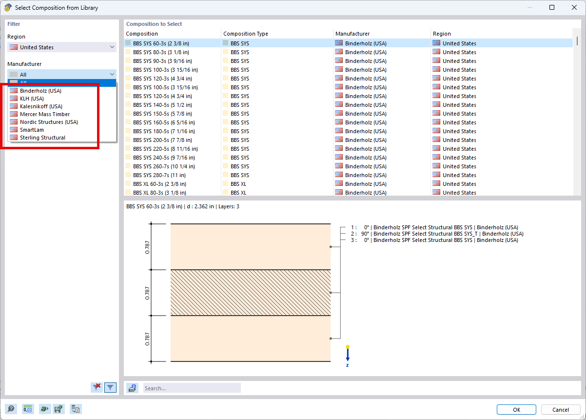
Among others, the following cross-laminated timber manufacturers are available in the layer structure library:
- Binderholz (USA)
- KLH (USA, CAN)
- Kalesnikoff (USA, CAN)
- Nordic Structures (USA, CAN)
- Mercer Mass Timber
- SmartLam
- Sterling Structural
- Superstructures listed in Lignatec Edition 32 "Cross-Laminated Timber of Swiss Production"
By importing a structure from the layer structure library, all relevant parameters are adopted automatically. The library is continually updated.
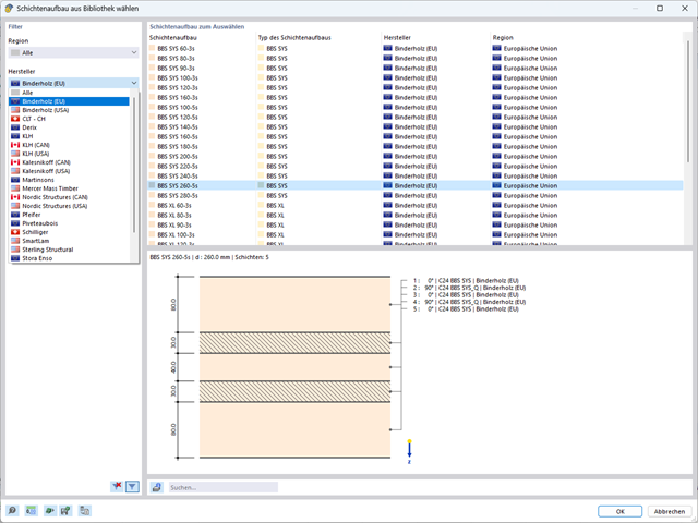
A library for cross-laminated timber panels is implemented in RFEM, from which you can import the manufacturer's layer structures (for example, Binderholz, KLH, Piveteaubois, Södra, Züblin Timber, Schilliger, Stora Enso). In addition to the layer thicknesses and materials, there is also the information about stiffness reductions and the narrow side bonding.
Go to Explanatory Video.png?mw=640&hash=55038d2a1591f62179796666cb9b2fede0274e19)
A graphical and tabular output of the results for deformations, stresses, and strains helps you when determining the soil solids. To achieve this, use the special filter criteria for targeted selection of results.
The program doesn't leave you alone with the results. If you want to graphically evaluate the results in the soil solids, you can use the guide objects. For example, you can define clipping planes. This allows you to view the corresponding results in any plane of the soil solid.
And not just that. The utilization of result sections and clipping boxes facilitates the precise graphical analysis of the soil solid.
You already know that it is possible to model and analyze a soil and a structure in the entire model. As a result, you have explicitly taken into account the soil-structure interaction. By modifying a component, you achieve the immediate correct consideration in the analysis as well as in the results for the entire system of the soil and structure.

Are you ready for the evaluation? Use the calculation diagrams, which show the distribution of a specific result during the calculation.
You can freely define the layout of the vertical and horizontal axes of the calculation diagram. This allows you, for example, to consider the settlement distribution of a certain node, depending on the load.

Your data are always documented in a multilingual printout report. You can adjust the content at any time and save it as a template. You can also add graphics, texts, MathML formulas, and PDF documents to your report with just a few clicks.
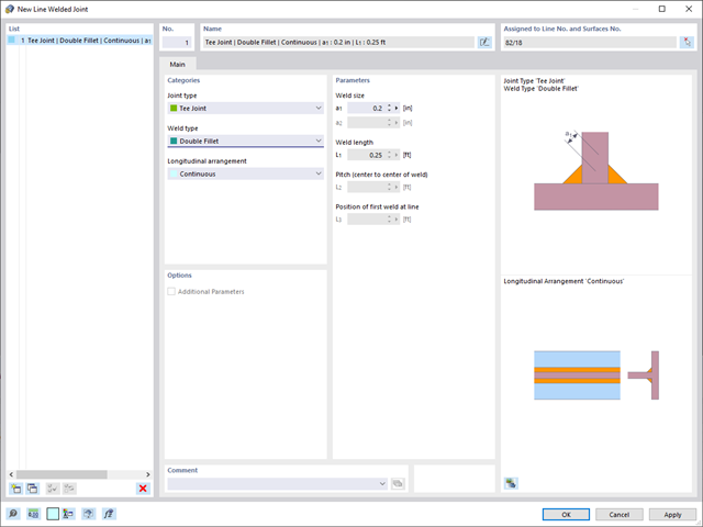
In RFEM 6, it is possible to define line welds between surfaces and to calculate the weld stresses using the Stress-Strain Analysis add-on.
The following joint types are available:
- Butt Joint
- Corner joint
- Lap Joint
- T-joint
Depending on the selected joint type, you can select the following weld types:
- Single Square
- Double Square
- Double Bevel
- Single V
- Double V
- Single U
- Double U
- Single J
- Double J

Enter and model a soil solid directly in RFEM. You can combine the soil material models with all common RFEM add-ons.
This allows you to easily analyze the entire models with a complete representation of the soil-structure interaction.
All parameters required for the calculation are automatically determined from the material data that you have entered. The program then generates the stress-strain curves for each FE element.

Did you know? You can enter the soil layers that you have obtained from the subsoil expertises done in the locations into the program in the form of soil samples. Assign the explored soil materials, including their material properties, to the layers.
For the definition of the samples, you can enter the data in tables as well as in the respective editing dialog box. Furthermore, you can also specify the groundwater level in the soil samples.

The soil solids that you want to analyze are summarized in soil massifs.
Use the soil samples as a basis for a definition of the respective soil massif. This way, the program allows for user-friendly generation of the massif, including the automatic determination of the layer interfaces from the sample data, as well as the groundwater level and the boundary surface supports.
Soil massifs provide you with the option to specify a target FE mesh size independently of the global setting for the rest of the structure. You can thus consider the various requirements of the building and soil in the entire model.

Do you want to model and analyze the behavior of a soil solid? To ensure this, special suitable material models have been implemented in RFEM.
You can use the modified Mohr-Coulomb model with a linear-elastic ideal-plastic model or a nonlinear elastic model with an oedometric stress-strain relation. The limit criterion, which describes the transition from the elastic area to that of the plastic flow, is defined according to Mohr-Coulomb.

The stress and strain results by surface can be output in the surface result table according to the thickness layer.

- 002232
- General
- Optimization & Cost / CO2 Emission Estimation for RFEM 6
- Optimization & Cost / CO2 Emission Estimation for RSTAB 9
You can be sure that costs are an important factor in the structural planning of any project. It is also essential to adhere to the provisions on emissions estimation. The two-part add-on Optimization & Costs/CO2 Emission Estimation makes it easier for you to find your way through the jungle of standards and options. It uses the artificial intelligence technology (AI) of the particle swarm optimization (PSO) to find the right parameters for parameterized models and blocks that guarantee the compliance with the usual optimization criteria. This add-on also estimates the model costs or CO2 emissions by specifying unit costs or emissions per material definition for the structural model. With this add-on, you are on the safe side.

Do you have great respect for the ravages of time? After all, it eventually gnaws at your construction projects. Use the Time-Dependent Analysis (TDA) add-on to consider the time-dependent material behavior of members. Long-term effects, such as creep, shrinkage, and aging, can influence the distribution of internal forces, depending on the structure. Prepare for this optimally with this add-on.
For each load case, the deformations can be displayed at the end time.
These results are also documented for you in the printout report of RFEM and RSTAB. You can select the report contents and extent specifically for the individual design checks.

Compared to the RF-/STEEL Warping Torsion add-on module (RFEM 5 / RSTAB 8), the following new features have been added to the Torsional Warping (7 DOF) add-on for RFEM 6 / RSTAB 9:
- Complete integration into the environment of RFEM 6 and RSTAB 9
- 7th degree of freedom is directly taken into account in the calculation of members in RFEM/RSTAB on the entire system
- No more need to define support conditions or spring stiffnesses for calculation on the simplified equivalent system
- Combination with other add-ons is possible, for example for the calculation of critical loads for torsional buckling and lateral-torsional buckling with stability analysis
- No restriction to thin-walled steel sections (it is also possible to calculate ideal overturning moments for beams with massive timber sections, for example)

Compared to the RF‑SOILIN add-on module (RFEM‑5), the following new features have been added to the Geotechnical Analysis add-on for RFEM 6:
- Creation of the layered soil as a 3D model from the entirety of the defined soil samples
- Recognized material law according to Mohr-Coulomb for soil simulation
- Graphical and tabular output of stresses and strains at any depth of the soil
- Optimal consideration of the soil-structure interaction on the basis of an overall model

Compared to the RF‑/STEEL add-on module (RFEM 5 / RSTAB 8), the following new features have been added to the Stress-Strain Analysis add-on for RFEM 6 / RSTAB 9:
- Treatment of members, surfaces, solids, welds (line welded joints between two and three surfaces with subsequent stress design)
- Output of stresses, stress ratios, stress ranges, and strains
- Limit stress depending on the assigned material or a user-defined input
- Individual specification of the results to be calculated through freely assignable setting types
- Non-modal result details with prepared formula display and additional result display on the cross-section level of members
- Output of the design check formulas used

Compared to the RF‑/STABILITY (RFEM 5) and RSBUCK (RSTAB 8) add-on modules, the following new features have been added to the Structure Stability add-on for RFEM 6 / RSTAB 9:
- Activation as a property of a load case or a load combination
- Automated activation of the stability calculation via combination wizards for several load situations in one step
- Incremental load increase with user-defined termination criteria
- Modification of the mode shape normalization without recalculation
- Result tables with filter option

- 002108
- General
- Optimization & Cost / CO2 Emission Estimation for RFEM 6
- Optimization & Cost / CO2 Emission Estimation for RSTAB 9
- Artificial intelligence technology (AI): Particle swarm optimization (PSO)
- Structure optimization according to the minimum weight or deformation
- Use of any number of optimization parameters
- Specification of variable ranges
- Optimization of cross-sections and materials
- Parameter definition types
- Optimization | Ascending or Optimization | Descending
- Application of parametric models and blocks
- Code-based JavaScript parametrization of blocks
- Optimization taking into account the design results
- Tabular display of the best model mutations
- Real-time display of the model mutations in the optimization process
- Model cost estimation by specifying unit prices
- Determination of the global warming potential GWP when realizing the model by estimating the CO2 equivalent
- Specification of weight-, volume-, and area-based units (price and CO2e)

- 002109
- General
- Optimization & Cost / CO2 Emission Estimation for RFEM 6
- Optimization & Cost / CO2 Emission Estimation for RSTAB 9
Did you know? The structural optimization in the programs RFEM and RSTAB is a completion of the parametric input. It is a parallel process beside the actual model calculation with all its regular calculation and design definitions. The add-on assumes that your model or block is built with a parametric context and is controlled in its entirety by global control parameters of the "optimization" type. Therefore, these control parameters have a lower and upper limit and a step size to delimit the optimization range. If you want to find optimal values for the control parameters, you have to specify an optimization criterion (for example, minimum weight) with the selection of an optimization method (for example, particle swarm optimization).
You can already find the cost and CO2 emission estimation in the material definitions. You can activate both options individually in each material definition. The estimation is based on a unit for unit cost or unit emission for members, surfaces, and solids. In this case, you can select whether to specify the units by weight, volume, or area.

- 002110
- General
- Optimization & Cost / CO2 Emission Estimation for RFEM 6
- Optimization & Cost / CO2 Emission Estimation for RSTAB 9
There are two methods that you can use for the optimization process, with which you can find optimal parameter values according to a weight or deformation criterion.
The most efficient method with the littlest calculation time is the near-natural particle swarm optimization (PSO). Have you heard or read about it? This artificial intelligence (AI) technology has a strong analogy to the behavior of flocks of animals, looking for a resting place. In such swarms, you can find many individuals (cf. optimization solution - for example, weight) who like to stay in a group and follow the group movement. Let's assume that each individual swarm member has a need to rest at an optimal resting place (cf. best solution - for example, lowest weight). This need increases as the resting place is approached. Thus, the swarm behavior is also influenced by the properties of the space (cf. result diagram).
Why the excursion into biology? Quite simply – the PSO process in RFEM or RSTAB proceeds in a similar way. The calculation run starts with an optimization result from a random assignment of the parameters to be optimized. It repeatedly determines new optimization results with varied parameter values, which are based on the experience of the previously performed model mutations. The process continues until the specified number of possible model mutations is reached.
As an alternative to this method, the program also offers you a batch processing method. This method attempts to check all possible model mutations by randomly specifying the values for the optimization parameters until a predetermined number of possible model mutations is reached.
After calculating a model mutation, both variants also check the respective activated design results of the add-ons. Furthermore, they save the variant with the corresponding optimization result and value assignment of the optimization parameters if the utilization is < 1.
You can determine the estimated total costs and emission from the respective sums of the individual materials. The sums of the materials are composed of the weight-based, volume-based, and area-based partial sums of the member, surface, and solid elements.

- 002161
- General
- Optimization & Cost / CO2 Emission Estimation for RFEM 6
- Optimization & Cost / CO2 Emission Estimation for RSTAB 9
Both optimization methods have one thing in common. At the end of the process, they provide you with a list of model mutations from the stored data. Here you can find the details of the controlling optimization result and the associated value assignment of the optimization parameters. This list is organized in descending order. You can find the assumed best solution shown in the first line. For this, the optimization result with its determined value assignment is closest to the optimization criterion. All add-on results have a utilization < 1. Furthermore, once the analysis is completed, the program will adjust the value assignment to that of the optimal solution for the optimization parameters in the global parameter list.
In the material dialog boxes, you can find the additional tabs "Cost Estimation" and "Estimation of CO2 Emissions". They show you the individual estimated sums of the assigned members, surfaces, and solids per unit weight, volume, and area. Furthermore, these tabs show the total cost and emission of all assigned materials. This gives you a good overview of your project.
_ENG.png?mw=640&hash=1053c9bef400e9f5361c9c3278f76a272fcc4ddf)
Have you activated the Time-Dependent Analysis (TDA) add-on? Very well, now you can add time data to load cases. After you have defined the start and end of the load, the influence of creep at the end of the load is taken into account. The program allows you to model creep effects for frame and truss structures made of reinforced concrete.
In this case, the calculation is performed nonlinearly according to the rheological model (Kelvin and Maxwell model).
Was the calculation successful? You can now display the determined internal forces in tables and graphics, and consider them in the design.

- Realistic representation of interaction between a building and soil
- Realistic representation of the influences of the foundation components on each other
- Extensible library of soil properties
- Consideration of several soil samples (probes) at different locations, even outside the building
- Determination of settlements and stress diagrams as well as their graphical and tabular display
Entering soil layers for soil samples is performed in a clearly arranged dialog box. A corresponding graphical representation supports clarity and makes checking the input user-friendly.
An extensible database facilitates the selection of soil material properties. The Mohr-Coulomb model as well as a nonlinear model with stress and strain dependent stiffness are available for a realistic modeling of the soil material behavior.
You can define any number of soil samples and layers. The soil is generated from all entered samples using 3D solids. Assignment to the structure is carried out using coordinates.
The soil body is calculated according to the nonlinear iterative method. The calculated stresses and settlements are displayed graphically and in tables.

- Calculation of models consisting of member, shell, and solid elements
- Nonlinear stability analysis
- Optional consideration of axial forces from initial prestress
- Four equation solvers for an efficient calculation of various structural models
- Optional consideration of stiffness modifications in RFEM/RSTAB
- Determination of a stability mode greater than the user-defined load increment factor (Shift method)
- Optional determination of the mode shapes of unstable models (to identify the cause of instability)
- Visualization of the stability mode
- Basis for determining imperfection