
In the Stress-Strain Analysis add-on, you can define a component-dependent limit stress cycle and consider it for the design.

In the ultimate configuration of the steel joint design, you have the option to modify the limit plastic strain for welds.

The "Base Plate" component allows you to design base plate connections with cast-in anchors. In this case, plates, welds, anchorages, and steel-concrete interaction are analyzed.

In the Geotechnical Analysis add-on, the Hoek-Brown material model is available. The model shows linear-elastic ideal-plastic material behavior. Its nonlinear strength criterion is the most common failure criterion for stone and rocks.
You can enter the material parameters using
- Rock parameters directly, or alternatively via
- GSI classification.
Detailed information about this material model and the definition of the input in RFEM can be found in the respective chapter Hoek-Brown Model of the online manual for the Geotechnical Analysis add-on.

The parameters of the National Annexes (NA) to Eurocode 3 of the following countries are integrated:
-
 DIN EN 1993-1-1/NA:2016-04 (Germany)
 -
 ÖNORM EN 1993-1-1/NA:2015-12 (Austria)
 -
 SN EN 1993-1-1/NA:2016-07 (Switzerland)
 -
 BDS EN 1993-1-1/NA:2015-10 (Bulgaria)
 -
 BS EN 1993-1-1/NA:2016-07 (United Kingdom)
 -
 CEN EN 1993-1-1/2015-06 (European Union)
 -
 CYS EN 1993-1-1/NA:2015-07 (Cyprus)
 -
 CSN EN 1993-1-1/NA:2016-06 (Czech Republic)
 -
 DS EN 1993-1-1/NA:2015-07 (Denmark)
 -
 ELOT EN 1993-1-1/NA:2017-01 (Greece)
 -
 EVS EN 1993-1-1/NA:2015-08 (Estonia)
 -
 HRN EN 1993-1-1/NA:2016-03 (Croatia)
 -
 I S. EN 1993-1-1/NA:2016-03 (Ireland)
 -
 ILNAS EN 1993-1-1/NA:2015-06 (Luxembourg)
 -
 IST EN 1993-1-1/NA:2015-11 (Iceland)
 -
 LST EN 1993-1-1/NA:2017-01 (Lithuania)
 -
 LVS EN 1993-1-1/NA:2015-10 (Latvia)
 -
 MS EN 1993-1-1/NA:2010-01 (Malaysia)
 -
 MSZ EN 1993-1-1/NA:2015-11 (Hungary)
 -
 NBN EN 1993-1-1/NA:2015-07 (Belgium)
 -
 NEN EN 1993-1-1/NA:2016-12 (Netherlands)
 -
 NF EN 1993-1-1/NA:2016-02 (France)
 -
 NP EN 1993-1-1/NA:2009-03 (Portugal)
 -
 NS EN 1993-1-1/NA:2015-09 (Norway)
 -
 PN EN 1993-1-1/NA:2015-08 (Poland)
 -
 SFS EN 1993-1-1/NA:2015-08 (Finland)
 -
 SIST EN 1993-1-1/NA:2016-09 (Slovenia)
 -
 SR EN 1993-1-1/NA:2016-04 (Romania)
 -
 SS EN 1993-1-1/NA:2019-05 (Singapore)
 -
 SS EN 1993-1-1/NA:2015-06 (Sweden)
 -
 STN EN 1993-1-1/NA:2015-10 (Slovakia)
 -
 TKP EN 1993-1-1/NA:2015-04 (Belarus)
 -
 UNE EN 1993-1-1/NA:2016-02 (Spain)
 -
 UNI EN 1993-1-1/NA:2015-08 (Italy)
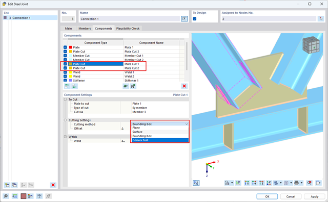
You can use the "Plate Cut" component to cut plates (for example, gusset plates, fin plates, and so on). There are various cutting methods available:
- Plane: The cut is performed on the closest surface to the reference plate.
- Surface: Only the intersecting parts of plates are cut.
- Bounding Box: The outermost dimension consisting of width and height is cut out of the plate as a rectangle.
- Convex Envelope: The outer hull of the cross-section is used for the plate cut. If there are fillets at the corner nodes of the cross-section, the cut is adapted to them.

- Realistic representation of interaction between a building and soil
- Realistic representation of the influences of the foundation components on each other
- Extensible library of soil properties
- Consideration of several soil samples (probes) at different locations, even outside the building
- Determination of settlements and stress diagrams as well as their graphical and tabular display
_(1).png?mw=640&hash=415f7bbaf70e41679bb0106e1cf91eaa8c493ec9)
- Automatic generation of FE analysis models: The add-on automatically creates a finite element model (FE) of the steel connection in the background.
- Consideration of all internal forces: The calculation and design checks include all internal forces (N, Vy, Vz, My, Mz, MT) and are not limited to planar loading.
- Automatic load transfer: All load combinations are automatically transferred to the FE analysis model of the connection. The loads are transferred directly from RFEM, so manual data input is not necessary.
- Efficient modeling: The add-on saves you time when modeling complex connection situations. You can also save the created FE analysis model and use it further for your own detailed analyses.
- Extensible library: An extensive and extensible library with predefined steel connection templates is available.
- Wide applicability: The add-on is suitable for connections of any type and shape, compatible with almost all rolled, welded, built-up, and thin-walled cross-sections.
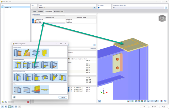
You can now insert a cap plate in steel joints with only a few clicks. You can enter the data using the known definition types "Offsets" or "Dimensions and Position". By specifying a reference member and the cutting plane, it is also possible to omit the Member Section component.
This component allows you to easily model cap plates on column ends, for example.

- Cross-section optimization
- Transfer of optimized sections to RFEM/RSTAB
- Design of any thin-walled section from RSECTION
- Representation of a stress diagram on a section
- Determination of normal, shear, and equivalent stresses
- Output of stress components for the individual member internal force types
- Detailed representation of stresses in all stress points
- Determination of the largest Δσ for each stress point (for example, for fatigue design)
- Colored display of stresses and design ratios for a quick overview of the critical or oversized zones
- Output of parts lists

Enter and model a soil solid directly in RFEM. You can combine the soil material models with all common RFEM add-ons.
This allows you to easily analyze the entire models with a complete representation of the soil-structure interaction.
All parameters required for the calculation are automatically determined from the material data that you have entered. The program then generates the stress-strain curves for each FE element.

The modal relevance factor (MRF) can help you to assess to which extent specific elements participate in a specific mode shape. The calculation is based on the relative elastic deformation energy of each individual member.
The MRF can be used to distinguish between local and global mode shapes. If multiple individual members show significant MRF (for example, > 20%), the instability of the entire structure or a substructure is very likely. On the other hand, if the sum of all MRFs for an eigenmode is around 100%, a local stability phenomenon (for example, buckling of a single bar) can be expected.
Furthermore, the MRF can be used to determine critical loads and equivalent buckling lengths of certain members (for example, for stability design). Mode shapes for which a specific member has small MRF values (for example, < 20%) can be neglected in this context.
The MRF is displayed by mode shape in the result table under Stability Analysis → Results by Members → Effective Lengths and Critical Loads.
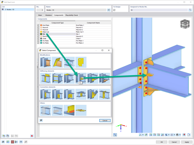
Using the "Rib" component, you can define any number of longitudinal ribs on a member plate. By defining a reference object, you can automatically specify welds on it.
The "Rib" component can also be arranged on circular hollow sections. Dafür wird zusätzlich die Vorgabe der Winkel zwischen den Rippen benötigt.

- General stress analysis
- Automatic import of internal forces from RFEM/RSTAB
- Graphical and numerical output of stresses, strains, clearance, and design ratios fully integrated in RFEM/RSTAB
- User-defined specification of the limit stress
- Summary of similar structural components for the design
- Wide range of customization options for graphical output
- Clearly arranged result tables for a quick overview after the design
- Simple traceability of the results due to the complete documentation of the calculation method including all formulas
- High productivity due to the minimal amount of input data required
- Flexibility due to detailed setting options for basis and extent of calculations
- Gray zone display for unimportant value ranges (see Product Feature)

- Calculation of models consisting of member, shell, and solid elements
- Nonlinear stability analysis
- Optional consideration of axial forces from initial prestress
- Four equation solvers for an efficient calculation of various structural models
- Optional consideration of stiffness modifications in RFEM/RSTAB
- Determination of a stability mode greater than the user-defined load increment factor (Shift method)
- Optional determination of the mode shapes of unstable models (to identify the cause of instability)
- Visualization of the stability mode
- Basis for determining imperfection

The stress and strain results by surface can be output in the surface result table according to the thickness layer.
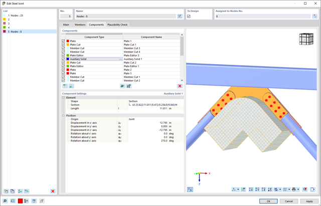
In the Steel Joints add-on, you can perform precise cuts on plates and structural components using the "Auxiliary Solid" component. Within this component, you can use the shapes of a box, a cylinder, or any cross-section as a guide object.
Go to Explanatory Video
- Selection of nodes in the RFEM model, automatic recognition and assignment of the members connected to the node
- Many predefined components available for easy input of typical connection situations (for example, end plates, cleats, fin plates)
- Universally applicable basic components (plates, welds, auxiliary planes) for entering complex connection situations
- No manual editing of the FE model required by the user, the essential calculation settings can be changed via the configuration settings
- Automatic adaptation of the connection geometry, even if the members are subsequently edited, due to the relative relation of the components to each other
- Parallel to the input, a plausibility check is carried out by the program to quickly detect missing input or collisions, for example
- Graphical display of the connection geometry that is updated in parallel with the input

If there is a load case or load combination in the program, the stability calculation is activated. You can define another load case in order to consider initial prestress, for example.
For this, you need to specify whether to perform a linear or nonlinear analysis. Depending on the case of application, you can select a direct calculation method, such as the Lanczos method or the ICG iteration method. Members not integrated in surfaces are usually displayed as member elements with two FE nodes. With such elements, the program cannot determine the local buckling of single members. That's why you have the option to divide members automatically.
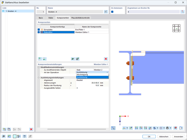
In the Member Editor component, you can also select the entire member as the modifying object instead of the individual member plates. This way, you can apply both operations "Notch" and "Chamfer" to several member plates.

Entering soil layers for soil samples is performed in a clearly arranged dialog box. A corresponding graphical representation supports clarity and makes checking the input user-friendly.
An extensible database facilitates the selection of soil material properties. The Mohr-Coulomb model as well as a nonlinear model with stress and strain dependent stiffness are available for a realistic modeling of the soil material behavior.
You can define any number of soil samples and layers. The soil is generated from all entered samples using 3D solids. Assignment to the structure is carried out using coordinates.
The soil body is calculated according to the nonlinear iterative method. The calculated stresses and settlements are displayed graphically and in tables.

Did you know? You can enter the soil layers that you have obtained from the subsoil expertises done in the locations into the program in the form of soil samples. Assign the explored soil materials, including their material properties, to the layers.
For the definition of the samples, you can enter the data in tables as well as in the respective editing dialog box. Furthermore, you can also specify the groundwater level in the soil samples.

- Determination of principal and basic stresses, membrane and shear stresses, as well as equivalent stresses and equivalent membrane stresses
- Stress analysis for structural surfaces including simple or complex shapes
- Equivalent stresses calculated according to different approaches:
- Shape modification hypothesis (von Mises)
- Shear stress hypothesis (Tresca)
- Normal stress hypothesis (Rankine)
- Principal strain hypothesis (Bach)
- Optional optimization of surface thicknesses and data transfer to RFEM
- Output of strains
- Detailed results of individual stress components and ratios in tables and graphics
- Filter function for solids, surfaces, lines, and nodes in tables
- Transversal shear stresses according to Mindlin, Kirchhoff, or user-defined specifications
- Stress evaluation for welds at connection lines between surfaces (see the Product Feature)

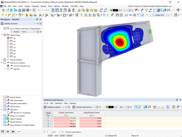
As the first results, the program presents you with the critical load factors. You can then perform an evaluation of stability risks. For member models, the resulting effective lengths and critical loads of the members are displayed to you in tables.
Use the next result window to check the normalized eigenvalues sorted by node, member, and surface. The eigenvalue graphic allows you to evaluate the buckling behavior. This makes it easier for you to take countermeasures.
You already know that it is possible to model and analyze a soil and a structure in the entire model. As a result, you have explicitly taken into account the soil-structure interaction. By modifying a component, you achieve the immediate correct consideration in the analysis as well as in the results for the entire system of the soil and structure.
.png?mw=640&hash=55038d2a1591f62179796666cb9b2fede0274e19)
A graphical and tabular output of the results for deformations, stresses, and strains helps you when determining the soil solids. To achieve this, use the special filter criteria for targeted selection of results.
The program doesn't leave you alone with the results. If you want to graphically evaluate the results in the soil solids, you can use the guide objects. For example, you can define clipping planes. This allows you to view the corresponding results in any plane of the soil solid.
And not just that. The utilization of result sections and clipping boxes facilitates the precise graphical analysis of the soil solid.
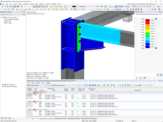
Do you work with steel connections? The Steel Joints add-on for RFEM supports you when analyzing steel connections by using an FE model. In this case, the modeling runs fully automatically in the background. Nevertheless, you can control this process via the simple and familiar input of components. You can then use the loads determined on the FE model for your design of the components according to EN 1993‑1‑8 (including National Annexes).
- The steel connections model and the results can be saved as a separate model file
- The resulting stresses and the results of the stability analysis (joint buckling) can be displayed in a separate model
- In the saved model, you can run a deformation animation on the connection
- Connection components are converted to surfaces and members when they are saved
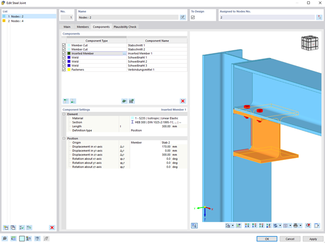
When designing connections, you can now also insert a new member as a component directly in the Steel Joints add-on. This will only be considered for the connection design. You can use the Weld and Fasteners components to connect to other members.
Furthermore, it is possible to use the Member Section and Member Editor components and arrange reinforcement elements on the inserted member, such as stiffeners and tapers.
Go to Explanatory VideoCompared to the RF‑/STABILITY (RFEM 5) and RSBUCK (RSTAB 8) add-on modules, the following new features have been added to the Structure Stability add-on for RFEM 6 / RSTAB 9:
- Activation as a property of a load case or a load combination
- Automated activation of the stability calculation via combination wizards for several load situations in one step
- Incremental load increase with user-defined termination criteria
- Modification of the mode shape normalization without recalculation
- Result tables with filter option