
The building model is calculated in two phases:
- Global 3D calculation of the global model, where the slabs are modeled as a rigid plane (diaphragm) or as a bending plate
- Local 2D calculation of the individual floors
After the calculation, the results of the columns and walls from the 3D calculation and the results of the slabs from the 2D calculation are combined in a single model. This means that there is no need to switch between the 3D model and the individual 2D models of the slabs. The user only works with one model, saves valuable time, and avoids possible errors in the manual data exchange between the 3D model and the individual 2D ceiling models.
The vertical surfaces in the model can be divided into shear walls and opening lintels. The program automatically generates internal result members from these wall objects, so they can be designed as members according to any standard in the Concrete Design add-on.
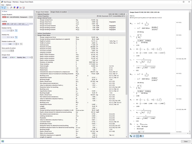
With Dlubal Software, you always have an overview, regardless of whether your projects are from the reinforced concrete, steel, timber, aluminum, or other industry. The program clearly displays the design check formulas used in your design (including a reference to the used equation from the standard). These design check formulas can also be included in the printout report.
Go to Explanatory Video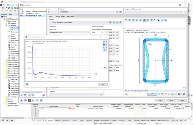
When performing a design according to EN 1993‑1‑3, it is possible to graphically display a mode shape for the distortional buckling of a cross-section, and for the RSECTION cross-sections.
The mode shape can also be output in RSECTION 1 for library cross-sections.

Have you activated the Building Model add-on? Very good! This allows you to display the center of rigidity in tabular and graphical form. Use it for your dynamic analysis, for example.

RFEM allows you to use a special line hinge to model the special properties of the connection between the reinforced concrete slab and masonry wall. This limits the transferable forces of the connection depending on the specified geometry. You guess right: This means that the material cannot be overloaded.
The program develops interaction diagrams that are applied automatically. They represent the various geometric situations and you can use them to determine the correct stiffness.
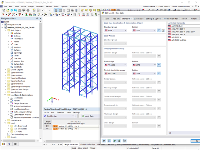
The design of cold-formed steel members according to the AISI S100-16 / CSA S136-16 is available in RFEM 6. Design can be accessed by selecting “AISC 360” or “CSA S16” as the standard in the Steel Design Add-on. “AISI S100” or “CSA S136” is then automatically selected for the cold-formed design.
RFEM applies the Direct Strength Method (DSM) to calculate the elastic buckling load of the member. The Direct Strength Method offers two types of solutions, numerical (Finite Strip Method) and analytical (Specification). The FSM signature curve and buckling shapes can be viewed under Sections.
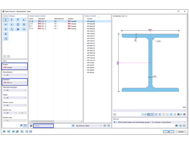
The new steel sections according to the latest CISC Handbook (12th edition) are available in RFEM 6. The sections are listed in the Standardized library. In the filter, select “Canada” for the region and “CISC 12” for the standard. Alternatively, the section name can be directly entered in the search box located at the bottom of the dialog box.

Are you ready for the evaluation? Use the calculation diagrams, which show the distribution of a specific result during the calculation.
You can freely define the layout of the vertical and horizontal axes of the calculation diagram. This allows you, for example, to consider the settlement distribution of a certain node, depending on the load.

Do you want to model and analyze the behavior of a soil solid? To ensure this, special suitable material models have been implemented in RFEM.
You can use the modified Mohr-Coulomb model with a linear-elastic ideal-plastic model or a nonlinear elastic model with an oedometric stress-strain relation. The limit criterion, which describes the transition from the elastic area to that of the plastic flow, is defined according to Mohr-Coulomb.
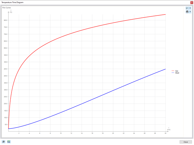
The governing component temperature at the time of analysis can be determined for the fire resistance design automatically using the input. In this case, you can follow the temperature curve in detail as a function of timeby displaying the temperature-time diagram.