
As you've already learned, the results of a Modal Analysis load case are displayed in the program after a successful calculation. You can thus immediately see the first mode shape graphically or as an animation. You can also easily adjust the representation of the mode shape standardization. Do that directly in the Results navigator, where you have one of four options for the visualization of the mode shapes available for the selection:
- Scaling the value of the mode shape vector uj to 1 (considers the translation components only)
- Selecting the maximum translational component of the eigenvector and setting it to 1
- Considering the entire eigenvector (including the rotation components), selecting the maximum, and setting it to 1
- Setting the modal mass mi for each mode shape to 1 kg
You can find a detailed explanation of the mode shape standardization in the OnlineManual here.

Is the calculation finished? The results of the modal analysis are then available both graphically and in tables. Display the result tables for the load case or the load cases of the modal analysis. Thus, you can see the eigenvalues, angular frequencies, natural frequencies, and natural periods of the structure at first glance. The effective modal masses, modal mass factors, and participation factors are also clearly displayed.

Are you ready for the evaluation? Use the calculation diagrams, which show the distribution of a specific result during the calculation.
You can freely define the layout of the vertical and horizontal axes of the calculation diagram. This allows you, for example, to consider the settlement distribution of a certain node, depending on the load.

Is your goal to determine the number of mode shapes? The program offers you two methods for this. On the one hand, you can manually define the number of the smallest mode shapes to be calculated. In this case, the number of available mode shapes depends on the degrees of freedom (that is, the number of free mass points multiplied by the number of directions in which the masses act). However, it is limited to 9999. On the other hand, you can set the maximum natural frequency the way that the program determined the mode shapes automatically until reaching the natural frequency set.
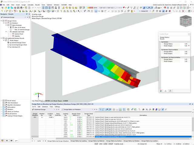
Did you use the eigenvalue solver of the add-on to determine the critical load factor within the stability analysis? In this case, you can then display the governing mode shape of the object to be designed as a result.
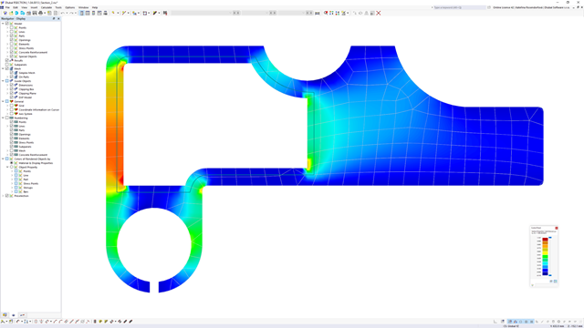
The Aluminum Design add-on provides you with further options. Here you can also design general cross-sections that are not predefined in the cross-section library. For example, create a cross-section in the RSECTION program and then import it into RFEM/RSTAB. Depending on the design standard used, you can select from various design formats. This includes, for example, the equivalent stress analysis.
With a license for RSECTION and Effective Sections, you can also perform the design checks while taking into account the effective cross-section properties according to EN 1993‑1‑5.

Do you want to model and analyze the behavior of a soil solid? To ensure this, special suitable material models have been implemented in RFEM.
You can use the modified Mohr-Coulomb model with a linear-elastic ideal-plastic model or a nonlinear elastic model with an oedometric stress-strain relation. The limit criterion, which describes the transition from the elastic area to that of the plastic flow, is defined according to Mohr-Coulomb.

Compared to the RF‑SOILIN add-on module (RFEM‑5), the following new features have been added to the Geotechnical Analysis add-on for RFEM 6:
- Creation of the layered soil as a 3D model from the entirety of the defined soil samples
- Recognized material law according to Mohr-Coulomb for soil simulation
- Graphical and tabular output of stresses and strains at any depth of the soil
- Optimal consideration of the soil-structure interaction on the basis of an overall model

The Concrete Design add-on allows you to perform the seismic design of reinforced concrete members according to EC 8. This includes, among other things, the following functionalities:
- Seismic design configurations
- Differentiation of the ductility classes DCL, DCM, DCH
- Option to transfer the behavior factor from a dynamic analysis
- Check of the limit value for the behavior factor
- Capacity design checks of "Strong column - weak beam"
- Detailing and particular rules for curvature ductility factor
- Detailing and particular rules for local ductility

The soil solids that you want to analyze are summarized in soil massifs.
Use the soil samples as a basis for a definition of the respective soil massif. This way, the program allows for user-friendly generation of the massif, including the automatic determination of the layer interfaces from the sample data, as well as the groundwater level and the boundary surface supports.
Soil massifs provide you with the option to specify a target FE mesh size independently of the global setting for the rest of the structure. You can thus consider the various requirements of the building and soil in the entire model.