- Design of five types of seismic force-resisting systems (SFRS) includes Special Moment Frame (SMF), Intermediate Moment Frame (IMF), Ordinary Moment Frame (OMF), Ordinary Concentrically Braced Frame (OCBF), and Special Concentrically Braced Frame (SCBF)
- Ductility check of the width-to thickness ratios for webs and flanges
- Calculation of the required strength and stiffness for stability bracing of beams
- Calculation of the maximum spacing for stability bracing of beams
- Calculation of the required strength at hinge locations for stability bracing of beams
- Calculation of the column required strength with the option to neglect all bending moments, shear, and torsion for overstrength limit state
- Design check of column and brace slenderness ratios
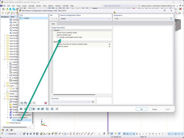
In the Concrete Design provides an option to perform seismic design according to AISC 341-16 for steel members.
Five SFRS types (Seismic Force-Resisting Systems) are available for this.
More Information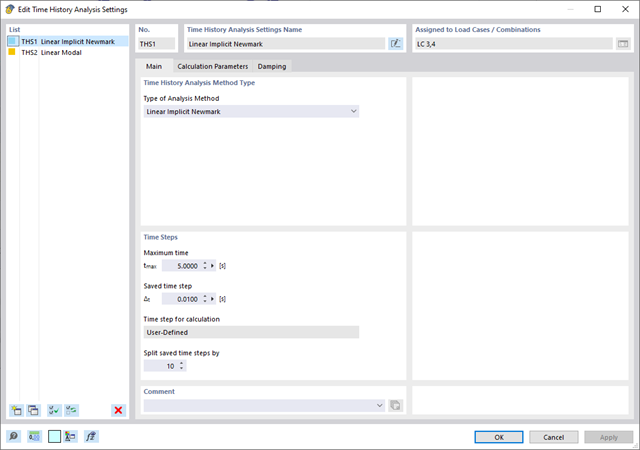
The time history analysis is performed with the modal analysis or the linear implicit Newmark analysis. The time history analysis in this add-on is limited to linear structural systems. Although the modal analysis represents a fast algorithm, it is necessary to use a certain number of eigenvalues to ensure the required accuracy of results.
The implicit Newmark analysis is a very precise method, independent of the number of eigenvalues used, but requires sufficient small time steps for the calculation.
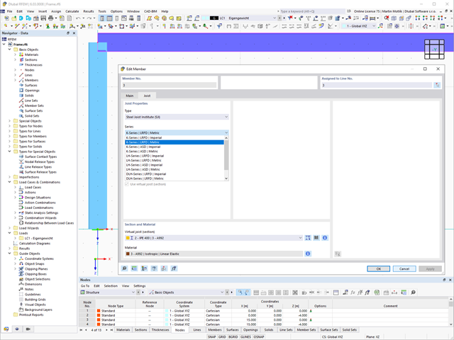
The "Virtual Joist" member type allows you to simulate prefabricated beams in a global model. The beam is replaced by a member with a virtual section.
This function makes it easier for you to simulate complex supporting units, such as a truss girder, in the overall system.
- Consideration of nonlinear component behavior using plastic standard hinges for steel (FEMA 356, EN 1998‑3) and nonlinear material behavior (masonry, steel - bilinear, user-defined working curves)
- Direct import of masses from load cases or combinations for the application of constant vertical loads
- User-defined specifications for the consideration of horizontal loads (standardized to a mode shape or uniformly distributed over the height of the masses)
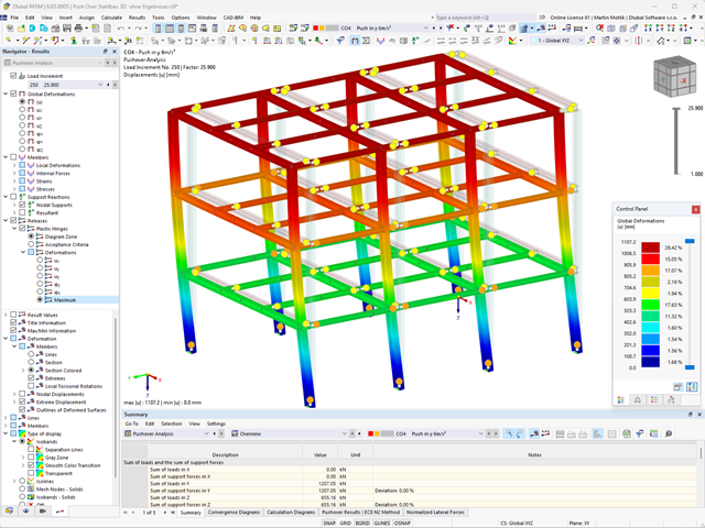
- Determination of a pushover curve with selectable limit criterion of the calculation (a collapse or limit deformation)
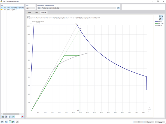
- Transformation of the pushover curve into the capacity spectrum (ADRS format, single degree of freedom system)
- Bilinearization of the capacity spectrum according to EN 1998‑1:2010 + A1:2013
- Transformation of the applied response spectrum into the required spectrum (ADRS format)
- Determination of target displacement according to EC 8 (the N2 method according to Fajfar 2000)
- Graphical comparison of the capacity and required spectrum
- Graphical evaluation of the acceptance criteria of predefined plastic hinges
- Result display of the values used in the iterative calculation of the target displacement
- Access to all results of the structural analysis in the individual load levels
During the calculation, the selected horizontal load is increased in load steps. A static nonlinear analysis is carried out for each load step until reaching the specified limit condition.
The results of the pushover analysis are extensive. On one hand, the structure is analyzed for its deformation behavior. This can be represented by a force-deformation line of the system (a capacity curve). On the other hand, the response spectrum effect can be displayed in the ADRS display (Acceleration-Displacement Response Spectrum). The target displacement is automatically determined in the program based on these two results. The process can be evaluated graphically and in tables.
The individual acceptance criteria can then be graphically evaluated and assessed (for the next load step of the target displacement, but also for all other load steps). The results of the static analysis are also available for the individual load steps.
You already know that it is possible to model and analyze a soil and a structure in the entire model. As a result, you have explicitly taken into account the soil-structure interaction. By modifying a component, you achieve the immediate correct consideration in the analysis as well as in the results for the entire system of the soil and structure.
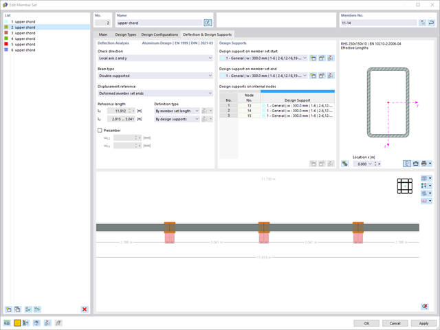
The program does a lot of work for you. For example, the load or result combinations required for the serviceability limit state are generated and calculated in RFEM/RSTAB. You can select these design situations for the deflection analysis in the Aluminum Design add-on. Depending on the specified precamber and reference system, the program determines the deformation values at each location of a member. They are then compared to the limit values.
You can specify the deformation limit value individually for each structural component in Serviceability Configuration. In this case, you define the maximum deformation depending on the reference length as the allowable limit value. By defining design supports, you can segment the components. In this way, you can determine the corresponding reference length automatically for each design direction.
And that's not all. Based on the position of the assigned design supports, the program allows you to automatically determine the distinction between beams and cantilevers. The limit value is thus determined accordingly.
As usual, you enter the structural system and calculate the internal forces in the programs RFEM and RSTAB. You have unlimited access to the extensive material and cross-section libraries. Did you know that you can create general cross-sections using the RSECTION program? That saves you a lot of work.
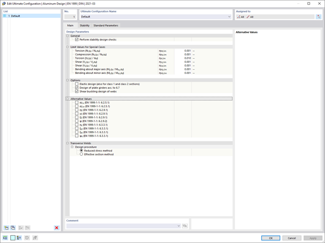
Don't be afraid of additional windows and input chaos! Aluminum Design is completely integrated into the main programs and automatically takes into account the structure and the available calculation results. You can directly assign further entries for the aluminum design, such as effective lengths, cross-section reductions, or design parameters, to the objects to be designed. You can simply and efficiently select the elements graphically using the [Select] function.

When defining the input data for the modal analysis load case, you can consider a load case whose stiffnesses represent the initial position for the modal analysis. How do you do that? As shown in the image, select the "Consider initial state from" option. Now, open the "Initial State Settings" dialog box and define the type Stiffness as the initial state. In this load case, as of which is the initial state taken into account, you can consider the stiffness of the structural system when the tension members fail. The purpose of all of this: The stiffness from this load case is considered in the modal analysis. Thus, you obtain a clearly flexible system.
.png?mw=640&hash=8b43c740f4a91092df759928a6ee21f06f78f8cc)
The calculation of masonry is carried out in compliance with the nonlinear-plastic material law. If the load at any point is higher than the possible load to be resisted, redistribution takes place within the system. This have the simple purpose of restoring the equilibrium of forces. With the successful completion of the calculation, the stability analysis is provided.
You can enter the structural system and calculate the internal forces in the programs RFEM and RSTAB. You have full access to the extensive material and cross-section libraries.
Timber Design is completely integrated into the main programs. At the same time, it automatically takes into account the structure and the available calculation results. You can assign further entries for the timber design, such as effective lengths, cross-section reductions, or design parameters, to the objects to be designed. You can easily select the elements graphically using the [Select] function at many places of the program.
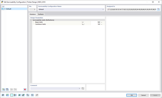
Your RFEM/RSTAB program is responsible for generating and calculating the load and result combinations required for the serviceability limit state. Select the design situations for the deflection analysis in the Timber Design add-on. The calculated deformation values are then determined at each location of a member, depending on the specified precamber and the reference system, and then compared to the limit values.
You can specify the deformation limit value individually for each structural component in Serviceability Configuration. In this case, the maximum deformation should not exceed the permissible limit value, depending on the reference length. When defining design supports, you can segment the components. This allows you to determine the corresponding reference length automatically for each design direction.
Based on the position of the assigned design supports, the program automatically determines the difference between beams and cantilevers. Thus, you can be sure that the limit value is determined accordingly.
In RFEM/RSTAB, you have the option to generate and then calculate the load or result combinations required for the serviceability limit state. You can select these design situations for the deflection analysis in the Steel Design add-on. The calculated deformation values are determined accordingly at each location of a member, depending on the specified precamber and reference system. Finaly, you can compare these deformation values with the limit values.
Did you know? You can specify the deformation limit value individually for each structural component in Serviceability Configuration. Define the maximum deformation depending on the reference length as the allowable limit value. By defining design supports, you can segment the components in order to determine the corresponding reference length automatically for each design direction.
Based on the position of the assigned design supports, the distinction between beams and cantilevers is made automatically so the limit value can be determined accordingly.
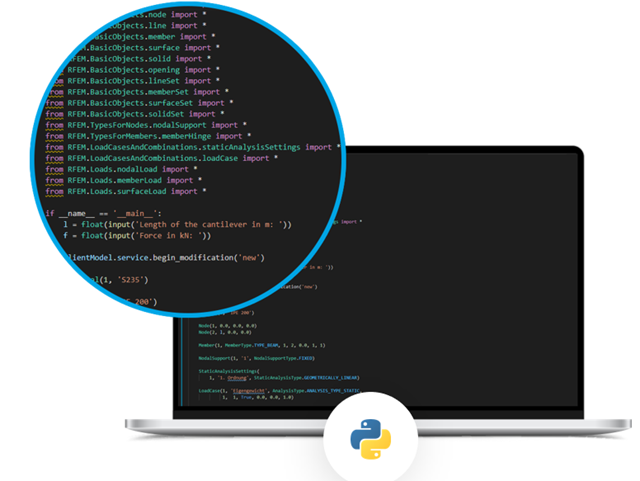
One thing is absolutely undisputed: WebService and API covers universal aspects in the construction industry. However, there is an issue. For the calculation and design, you need different features for each region, country, company, and civil engineer. Everyone has their own requirements. We have solved this problem. Since with WebService and API, you can easily create your very own calculation and design system. Always at your side: The performance and reliability of RFEM, RSTAB, and RSECTION.
The need for adapted and automated structural analysis and design is constantly increasing. WebService technology allows you to create special functionalities quickly and precisely. Our customers can develop such solutions independently or in cooperation with us. See for yourself and give it a try!
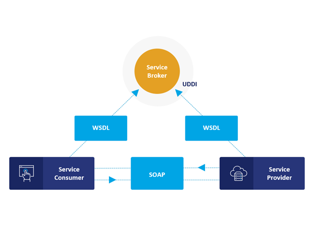
Communication is the key to success. This also applies to a client-server relation. WebService and API provides you with an XML based information exchange system for direct client-server communication. Programs, objects, messages, or documents can be integrated into these systems. For example, a web service protocol of the HTTP type runs for the client-server communication when you are looking for something in the Internet using a search engine.
Now back to Dlubal Software. In our case, the client is your programming environment (.NET, Python, JavaScript) and the service provider is RFEM 6. Client-server communication allows you to send requests to and receive feedback from RFEM, RSTAB, or RSECTION.
What is the difference between WebService and an API?
- WebService is a collection of open source protocols and standards used to exchange data between systems and applications. In contrast, an application programming interface (API), is a software interface through which two applications can interact without a user being involved.
- Thus, all web services are APIs, but not all APIs are web services.
What are the advantages of the WebService technology?
You can communicate more quickly within and between organizations.A service can be independent of other services.Webservice allows you to use your application to make your message or feature available to the rest of the world.Webservice helps you to exchange data between different applications and platforms Several applications can communicate, exchange data, and share services with each other. SOAP ensures that programs created on different platforms and based on different programming languages can exchange data securely.
Communication between the web service client and server is optionally encrypted via the https protocol. To do this, you can install an SSL certificate with the corresponding private key in the settings.
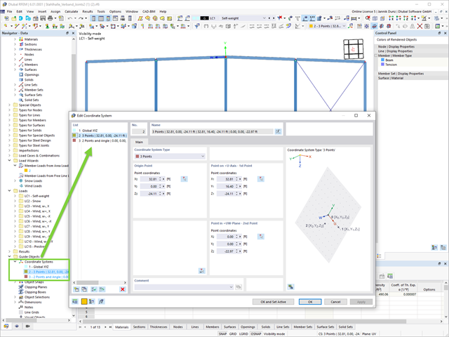
A change in favor of more efficient work withh the program: Your user-defined coordinate systems for input and analysis purposes are now organized globally under the guide objects.
Dlubal Software supports its customers with their construction planning worldwide. The modern online licensing system allows licenses of RFEM, RSTAB, and other programs to be distributed all over the world and assigned to the respective users via the Dlubal Account.
Go to Explanatory Video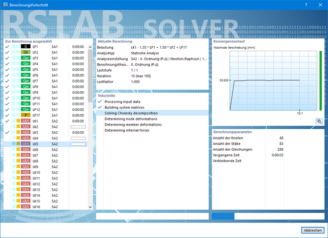
Also in this case, RSTAB will certainly convince you. With the powerful calculation kernel, its optimized networking and support of multi-core processor technology, the Dlubal structural analysis program is far ahead. This allows you to calculate more linear load cases and load combinations using several processors in parallel without using additional memory. The stiffness matrix only has to be created once. Thus, it is possible for you to calculate even large systems with the fast and direct solver.
Do you have to calculate multiple load combinations in your models? The program initiates several solvers in parallel (one per core). Each solver then calculates a load combination for you. This leads to better utilization of the cores.
You can systematically follow the development of the deformation displayed in a diagram during the calculation, and thus precisely evaluate the convergence behavior.

Compared to the RF-/STEEL Warping Torsion add-on module (RFEM 5 / RSTAB 8), the following new features have been added to the Torsional Warping (7 DOF) add-on for RFEM 6 / RSTAB 9:
- Complete integration into the environment of RFEM 6 and RSTAB 9
- 7th degree of freedom is directly taken into account in the calculation of members in RFEM/RSTAB on the entire system
- No more need to define support conditions or spring stiffnesses for calculation on the simplified equivalent system
- Combination with other add-ons is possible, for example for the calculation of critical loads for torsional buckling and lateral-torsional buckling with stability analysis
- No restriction to thin-walled steel sections (it is also possible to calculate ideal overturning moments for beams with massive timber sections, for example)

Once you activate the Form-Finding add-on in the Base Data, a form-finding effect is assigned to the load cases with the load case category "Prestress" in conjunction with the form-finding loads from the member, surface, and solid load catalog. This is a prestress load case. It thus mutates into a form-finding analysis for the entire model with all member, surface, and solid elements defined in it. You reach the form-finding of the relevant member and membrane elements amid the overall model by using special form-finding loads and regular load definitions. These form-finding loads describe the expected state of deformation or force after the form-finding in the elements. The regular loads describe the external loading of the entire system.
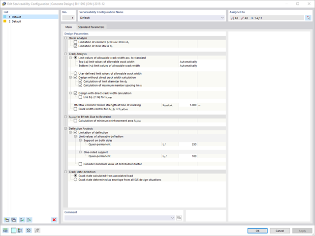
Are you looking for a deformation calculation? Check the Serviceability Configuration, where it can be activated. You can also control the consideration of long-term effects (creep and shrinkage) and tension stiffening between cracks in the dialog box above. The creep coefficient and shrinkage strain are calculated using the specified input parameters, or you can define them individually.
Furthermore, you can specify the deformation limit value individually for each structural component. The max. deformation is defined as the allowable limit value. In addition, you have to specify whether you want to use the undeformed or the deformed system for the design check.
The standards already specify the approximation methods (for example, deformation calculation according to EN 1992‑1‑1, 7.4.3, or ACI 318‑19, 24.3.2.5) that you need for your deformation calculation. In this case, the so-called effective stiffnesses are calculated in the finite elements in accordance with the existing limit state with / without cracks. You can then use these effective stiffnesses to determine the deformations by means of another FEM calculation.
Consider a reinforced concrete cross-section for the calculation of the effective stiffnesses of the finite elements. Based on the internal forces determined for the serviceability limit state in RFEM, you can classify the reinforced concrete cross-section as "cracked" or "uncracked". Do you consider the effect of the concrete between the cracks? In this case, this is done by means of a distribution coefficient (for example, according to EN 1992‑1‑1, Eq. 7.19, or ACI 318‑19, 24.3.2.5). You can assume the material behavior for the concrete to be linear-elastic in the compression and tension zone until reaching the concrete tensile strength. This procedure is sufficiently precise for the serviceability limit state.
When determining the effective stiffnesses, you can take into accout the creep and shrinkage at the "cross-section level." You don't need to consider the influence of shrinkage and creep in statically indeterminate systems in this approximation method (for example, tensile forces from shrinkage strain in systems restrained on all sides are not determined and have to be considered separately). In summary, the deformation calculation is carried out in two steps:
- Calculation of effective stiffnesses of the reinforced concrete cross-section assuming linear-elastic conditions
- Calculation of the deformation using the effective stiffnesses with FEM

If there are geometry differences arising between the ideal and the deformed structural system from the previous construction stage, they are compared in the program. The next construction stage is built on top of the stressed system from the previous construction stage. This calculation is nonlinear.
You enter the structural system and calculate the internal forces in the programs RFEM and RSTAB. You have full access to the extensive material and cross-section libraries. Did you know? You can also use the RSECTION program to create general cross-sections.
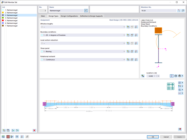
You find Steel Design fully integrated in the main programs. They automatically take into account the structure and the available calculation results. You can assign further entries for the aluminum design, such as effective lengths, cross-section reductions, or design parameters, to the objects to be designed. At many places of the program, you can easily select the elements graphically using the [Select] function.
You can perform the calculation of the warping torsion on the entire system. Thus, you consider the additional 7th degree of freedom in the member calculation. The stiffnesses of the connected structural elements are automatically taken into account. It means, you don't need to define equivalent spring stiffnesses or support conditions for a detached system.
You can then use the internal forces from the calculation with warping torsion in the add-ons for the design. Consider the warping bimoment and the secondary torsional moment, depending on the material and the selected standard. A typical application is the stability analysis according to the second-order theory with imperfections in steel structures.
Did you know that The application is not limited to thin-walled steel cross-sections. Thus, it is possible for you, for example, to perform the calculation of the ideal overturning moment of beams with solid timber cross-sections.
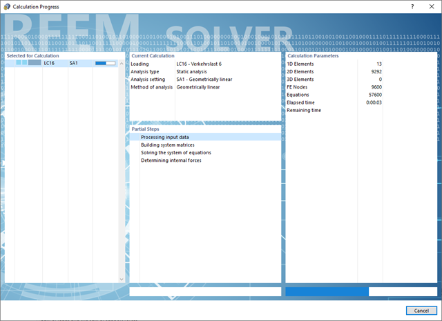
Convince yourself by the powerful calculation kernel, its optimized networking and support of multi-core processor technology. This provides you with the advantages, such as parallel calculations of linear load cases and load combinations using several processors without additional demands on the RAM. The stiffness matrix only has to be created once. Thus, you can calculate even large systems with the fast direct solver.
If you need to calculate multiple load combinations in your models, the program initiates several solvers in parallel (one per core). Each solver then calculates a load combination, which improves the core utilization.
You can systematically follow the development of the deformation displayed in a diagram during the calculation, and thus precisely evaluate the convergence behavior.
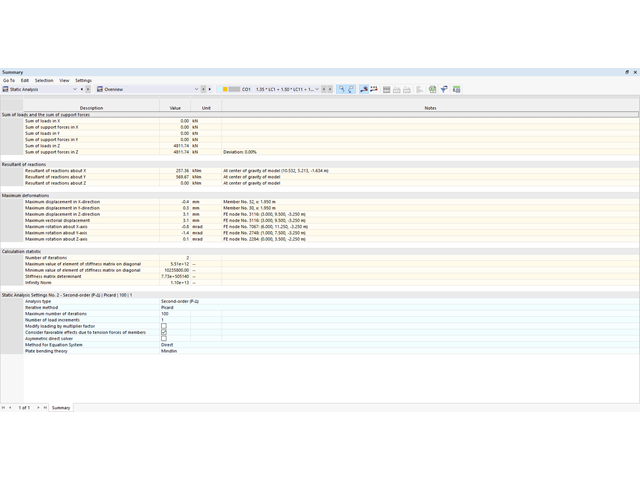
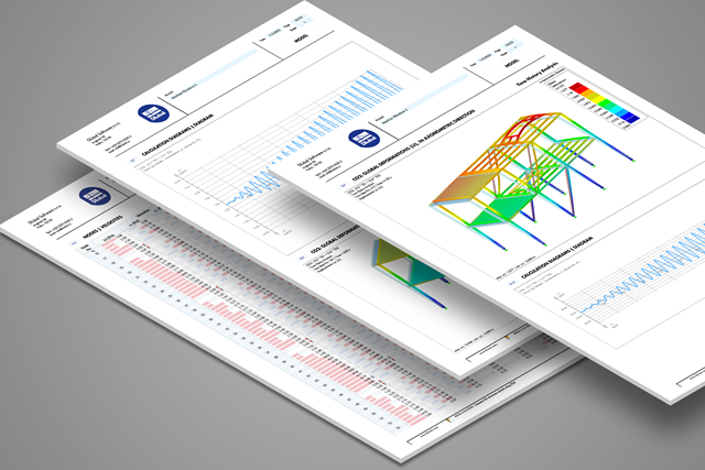
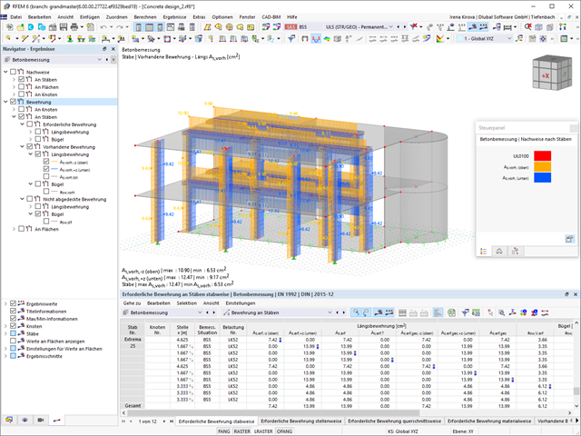
With clearly arranged tables, you can always keep an eye on your results. The first result table displays a summarized overview providing the equilibrium of forces in the structural system and the maximum deformations. Moreover, you also get the information about the calculation process. You can filter the result tables by specific criteria, such as extreme values or design locations, in order to obtain a better overview.
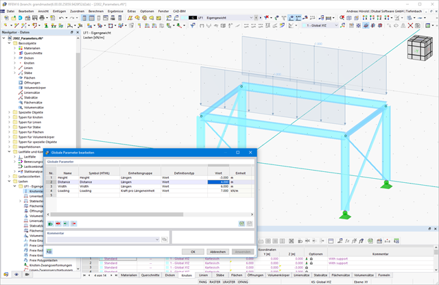
Do you want to efficiently process recurring systems? Then the parameterized input is recommended to you. You can create your models by using particular parameters and adjust them to a new situation by modifying the parameters.
If you want to manage recurring systems, you can use the parameterizable input. Models can be created using particular parameters and you can adjust them to a new situation by modifying the parameters.