
Get a better understanding of the stress distribution within member cross-sections by using clipping planes.
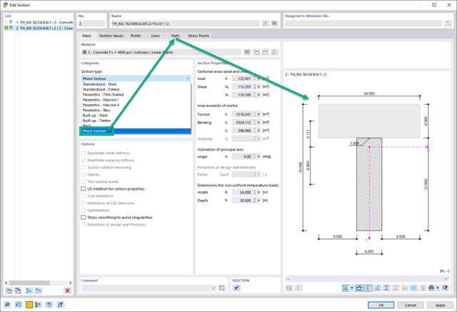
In the Construction Stages Analysis (CSA) add-on, you can use built-up cross-sections by means of what are known as phase sections. This allows you to activate and deactivate the parts of the "Parametric - Massive II" section type throughout the construction stages.
- Design of five types of seismic force-resisting systems (SFRS) includes Special Moment Frame (SMF), Intermediate Moment Frame (IMF), Ordinary Moment Frame (OMF), Ordinary Concentrically Braced Frame (OCBF), and Special Concentrically Braced Frame (SCBF)
- Ductility check of the width-to thickness ratios for webs and flanges
- Calculation of the required strength and stiffness for stability bracing of beams
- Calculation of the maximum spacing for stability bracing of beams
- Calculation of the required strength at hinge locations for stability bracing of beams
- Calculation of the column required strength with the option to neglect all bending moments, shear, and torsion for overstrength limit state
- Design check of column and brace slenderness ratios
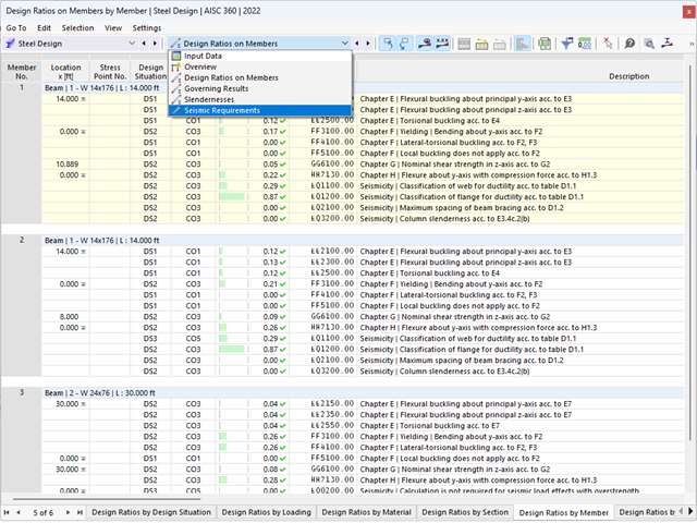
The seismic design result is categorized into two sections: member requirements and connection requirements.
The "Seismic Requirements" include the Required Flexural Strength and the Required Shear Strength of the beam-to-column connection for moment frames. They are listed in the ‘Moment Frame Connection by Member’ tab. For braced frames, the Required Connection Tensile Strength and the Required Connection Compressive Strength of the brace are listed in the ‘Brace Connection by Member’ tab.
The program provides the performed design checks in tables. The design check details clearly display the formulas and references to the standard.

In the Geotechnical Analysis add-on, the Hoek-Brown material model is available. The model shows linear-elastic ideal-plastic material behavior. Its nonlinear strength criterion is the most common failure criterion for stone and rocks.
You can enter the material parameters using
- Rock parameters directly, or alternatively via
- GSI classification.
Detailed information about this material model and the definition of the input in RFEM can be found in the respective chapter Hoek-Brown Model of the online manual for the Geotechnical Analysis add-on.
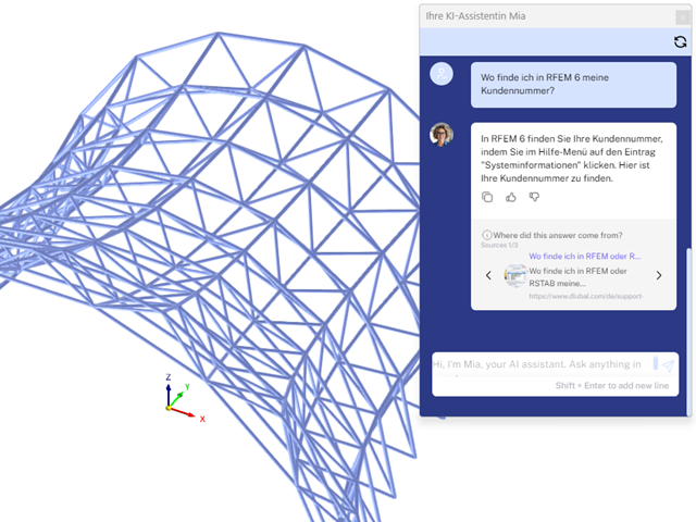
Mia is accessible in the programs and prevents the hassle of following up by email or phone.
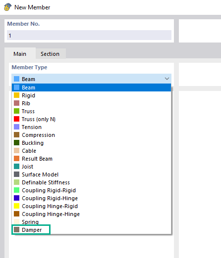
Using the "Damper" member type, you can define a damping coefficient, a spring constant, and a mass. This member type extends the possibilities within the Time History Analysis.
With regard to viscoelasticity, the "Damper" member type is similar to the Kelvin-Voigt model, which consists of the damping element and an elastic spring (both connected in parallel).

The building model is calculated in two phases:
- Global 3D calculation of the global model, where the slabs are modeled as a rigid plane (diaphragm) or as a bending plate
- Local 2D calculation of the individual floors
After the calculation, the results of the columns and walls from the 3D calculation and the results of the slabs from the 2D calculation are combined in a single model. This means that there is no need to switch between the 3D model and the individual 2D models of the slabs. The user only works with one model, saves valuable time, and avoids possible errors in the manual data exchange between the 3D model and the individual 2D ceiling models.
The vertical surfaces in the model can be divided into shear walls and opening lintels. The program automatically generates internal result members from these wall objects, so they can be designed as members according to any standard in the Concrete Design add-on.
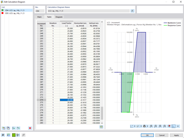
For calculation diagrams, you can use the "2D | Hinge" diagram type. These hinge diagrams show the hinge response of load situations for nonlinear hinges.
For calculations with several load situations, such as the case with the pushover analysis and time history analysis, you can evaluate the hinge condition in each load step.
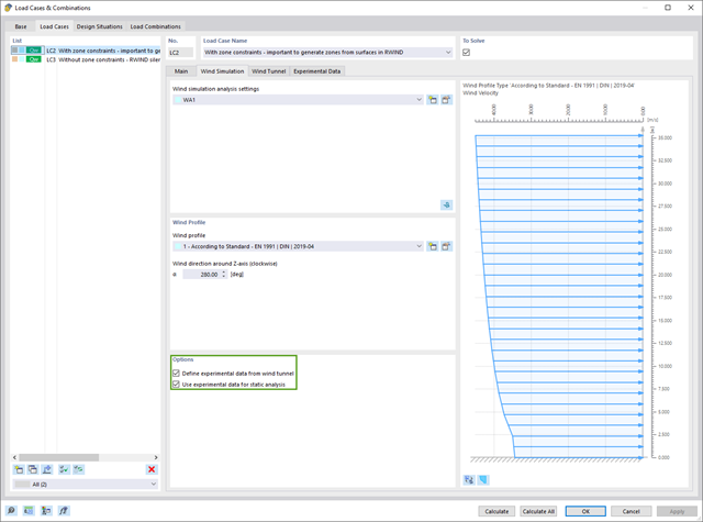
If you have experimentally determined surface pressures available for a model, you can apply them to a structural model in RFEM 6, process them in RWIND 2, and use them as wind loads in the structural analysis of RFEM 6.
You can find out how to apply the experimentally determined values in this technical article.

In the Modal Analysis add-on, you have the option to automatically increase the sought eigenvalues until reaching a defined effective modal mass factor. All translational directions activated as masses for the modal analysis are taken into account.
Thus, it is possible to easily calculate the required 90% of the effective modal mass for the response spectrum method.
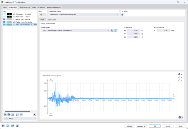
The Time History Analysis add-on provides you with accelerograms for the calculation. This extension allows for dynamic structural analysis of the acceleration-time diagrams.
There is an extensive library of earthquake records available for you, but you can also enter or import your own diagrams. The time history analysis is performed using the modal analysis or the linear implicit Newmark analysis.

For a response spectrum analysis of building models, you can display the sensitivity coefficients for the horizontal directions by story.
These key figures allow you to interpret the sensitivity to stability effects.

The modal relevance factor (MRF) can help you to assess to which extent specific elements participate in a specific mode shape. The calculation is based on the relative elastic deformation energy of each individual member.
The MRF can be used to distinguish between local and global mode shapes. If multiple individual members show significant MRF (for example, > 20%), the instability of the entire structure or a substructure is very likely. On the other hand, if the sum of all MRFs for an eigenmode is around 100%, a local stability phenomenon (for example, buckling of a single bar) can be expected.
Furthermore, the MRF can be used to determine critical loads and equivalent buckling lengths of certain members (for example, for stability design). Mode shapes for which a specific member has small MRF values (for example, < 20%) can be neglected in this context.
The MRF is displayed by mode shape in the result table under Stability Analysis → Results by Members → Effective Lengths and Critical Loads.
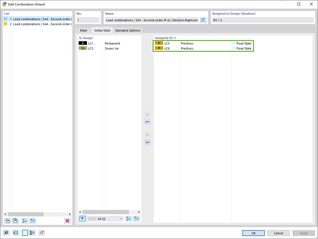
The combination wizard provides you with the option to consider more than one initial state. RFEM and RSTAB allow you to specify different initial states (prestress, form-finding, strain, and so on) for the target combinations in the combinatorics.
You can thus, for example, generate load states on the basis of a form-finding analysis with varying imperfections.
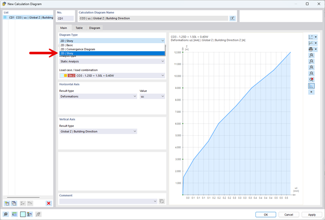
The "2D | Story" calculation diagram type is used to create result diagrams via the building axis. This allows you to easily analyze the behavior of the entire building under static and dynamic effects.
You can use this diagram type, for example, to visualize the seismic force over the building height.
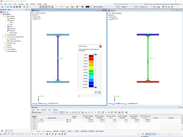
Within the "Plastic capacity design | Simplex Method" in RSECTION, the simultaneous variation of shear stresses over the cross-sectional area is performed in addition to the variation of axial stresses. This extended form of analysis allows you to use redistribution reserves, especially for the cross-sections subjected to shear loading, thus loading the cross-sections even more efficiently.
Go to Explanatory Video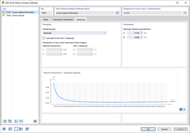
- Analysis of time diagrams and accelerograms (acceleration-time diagrams exciting the supports of a structure)
- Combination of user-defined time diagrams with nodal, member, and surface loads, as well as free and generated loads
- Combination of several independent excitation functions
- Linear implicit Newmark analysis or modal analysis in time history
- Structural damping using Raleigh damping coefficients or Lehr's damping value
- Graphical display of results in calculation diagrams
- Result display in individual time steps or as an envelope during the entire time period
- Extensive library of seismic events (accelerograms)
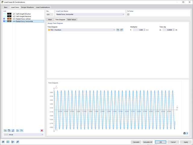
It is necessary to enter the required force-time diagrams. They can be combined in load cases or load combinations of the type Time History Analysis | Time Diagrams with the loading in order to define where and in which direction the force-time diagrams act.
The second option is to enter acceleration-time diagrams, which can be used in the load cases of the Time History Analysis | Accelerogram type.
All calculation parameters are specified in the time history analysis settings. These include, for example, the type of analysis method and the maximum calculation time.
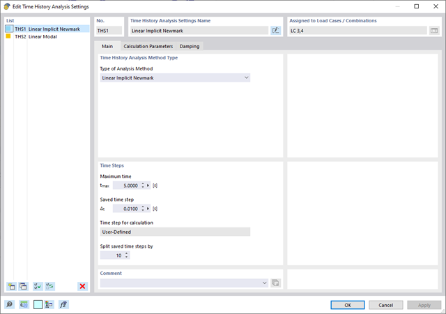
The time history analysis is performed with the modal analysis or the linear implicit Newmark analysis. The time history analysis in this add-on is limited to linear structural systems. Although the modal analysis represents a fast algorithm, it is necessary to use a certain number of eigenvalues to ensure the required accuracy of results.
The implicit Newmark analysis is a very precise method, independent of the number of eigenvalues used, but requires sufficient small time steps for the calculation.