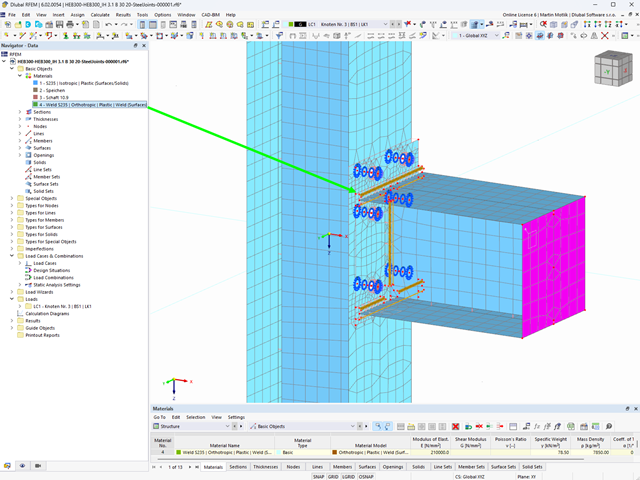
Here, the weld design becomes child's play. Using the specially developed material model "Orthotropic | Plastic | Weld (Surfaces)", you can calculate all stress components plastically. The stress τperpendicular is also considered plastically.
Using this material model you can design welds closer to reality and more efficiently.
Explanatory Video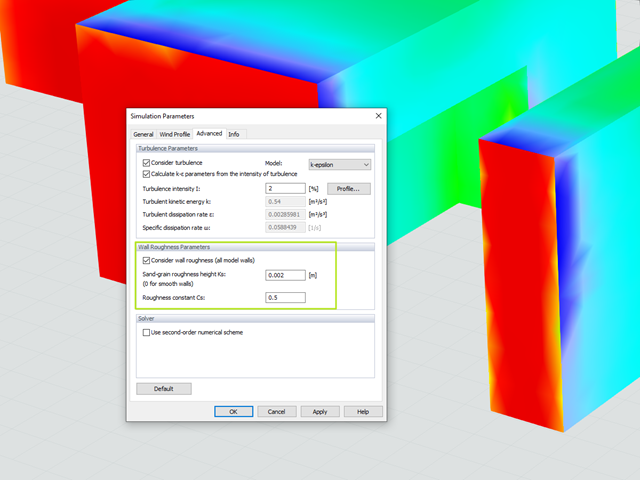
Utilize the RWIND Simulation program to consider a surface roughness of the model surface by applying a modified wall boundary condition. The numerical model is based on the assumption that grains with a certain diameter are arranged homogeneously on the model surface, similar to sandpaper. The grain diameter is described with the parameter Ks and the distribution with the parameter Cs. By considering the wall roughness, the numerical flow simulation can capture reality more closely.
SHAPE-THIN calculates all relevant cross‑section properties, including plastic limit internal forces. Overlapping areas are set close to reality. If cross-sections consist of different materials, SHAPE‑THIN determines the effective cross‑section properties with respect to the reference material.
In addition to the elastic stress analysis, you can perform the plastic design including interaction of internal forces for any cross‑section shape. The plastic interaction design is carried out according to the Simplex Method. You can select the yield hypothesis according to Tresca or von Mises.
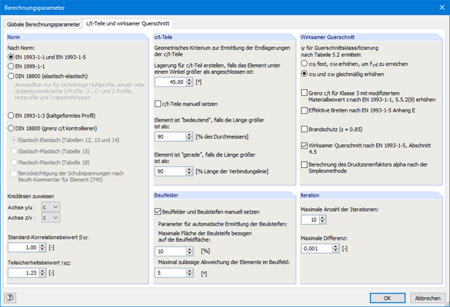
SHAPE-THIN performs a cross-section classification according to EN 1993-1-1 and EN 1999-1-1. For steel cross-sections of cross-section class 4, the program determines effective widths for unstiffened or stiffened buckling panels according to EN 1993-1-1 and EN 1993-1-5. For aluminum cross-sections of cross-section class 4, the program calculates effective thicknesses according to EN 1999-1-1.
Optionally, SHAPE‑THIN checks the limit c/t-values in compliance with the design methods el‑el, el‑pl, or pl‑pl according to DIN 18800. The c/t-zones of elements connected in the same direction are recognized automatically.
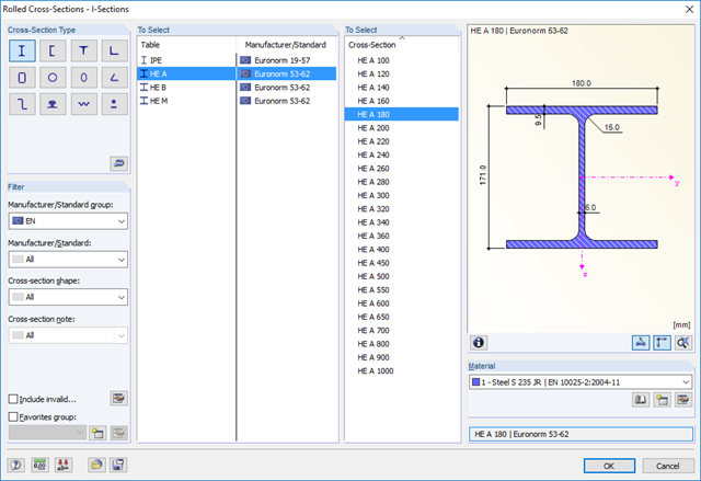
RF-/STEEL EC3 automatically imports the cross-sections defined in RFEM/RSTAB. It is possible to design all thin-walled cross-sections. The program automatically selects the most efficient method according to standards.
The ultimate limit state design takes into account several loads and you can select the interaction designs available in the standard.
The classification of designed cross-sections into Classes 1 to 4 is an essential part of the analysis according to Eurocode 3. This way, you can check the limitation of the design and rotational capacity by means of the local buckling of cross-section parts. RF-/STEEL EC3 determines the c/t-ratios of the cross-section parts subjected to compression stress and performs the classification automatically.
For the stability analysis, you can specify for each member or set of members whether flexural buckling occurs in the y- and/or the z-direction. You can also define additional lateral restraints in order to represent the model close to reality. The slenderness ratio and elastic critical load are determined automatically on the basis of the boundary conditions of RF-/STEEL EC3. The elastic critical moment for lateral-torsional buckling required for the lateral-torsional buckling analysis can be determined automatically or specified manually. The load application point of transverse loads, which has an influence on the torsional resistance, can also be taken into account via the setting in the details. In addition, you can take into account rotational restraints (for example trapezoidal sheeting and purlins) and shear panels (for example trapeziodal sheeting and bracing).
In modern construction, where cross-sections are increasingly slender, the serviceability limit state is an important factor in structural analysis. RF-/STEEL EC3 assigns load cases, load combinations, and result combinations to different design situations. The respective limit deformations are preset in the National Annex and can be adjusted, if necessary. In addition, it is possible to define reference lengths and precambers for the design.
Several methods are available for the eigenvalue analysis:
- Direct Methods
- The direct methods (Lanczos, roots of characteristic polynomial, subspace iteration method) are suitable for small to medium-sized models. These fast methods for equation solvers benefit from a lot of the computer memory (RAM). 64-bit systems use more memory so that even bigger structural systems can be calculated quickly.
- ICG iteration method (Incomplete Conjugate Gradient)
- This method requires only a small amount of memory. Eigenvalues are determined one after the other. It can be used to calculate large structural systems with few eigenvalues.
The RF-STABILITY add-on module can also perform the non-linear stability analysis. Also for nonlinear structures, results close to reality are provided. The critical load factor is determined by gradually increasing the loads of the underlying load case until the instability is reached. The load increment takes into account nonlinearities such as failing members, supports and foundations, and material nonlinearities.

You can select several methods that are available for the eigenvalue analysis:
- Direct Methods
- The direct methods (Lanczos [RFEM], roots of characteristic polynomial [RFEM], subspace iteration method [RFEM/RSTAB], and shifted inverse iteration [RSTAB]) are suitable for small to medium-sized models. You should only use these fast solver methods if your computer has a larger amount of memory (RAM).
- ICG Iteration Method (Incomplete Conjugate Gradient [RFEM])
- In contrast, this method only requires a small amount of memory. Eigenvalues are determined one after the other. It can be used to calculate large structural systems with few eigenvalues.
Use the Structure Stability add-on to perform a nonlinear stability analysis using the incremental method. This analysis delivers close-to-reality results also for nonlinear structures. The critical load factor is determined by gradually increasing the loads of the underlying load case until the instability is reached. The load increment takes into account nonlinearities such as failing members, supports and foundations, and material nonlinearities. After increasing the load, you can optionally perform a linear stability analysis on the last stable state in order to determine the stability mode.