
In the Stress-Strain Analysis add-on, you can define a component-dependent limit stress cycle and consider it for the design.

The Concrete Design add-on for RFEM allows you to perform the fire design of reinforced concrete walls and slabs according to the simplified table method (EN 1992‑1‑2, Section 5.4.2 and Table 5.8 and 5.9).

In the Concrete Design add-on, you have the option to define an existing vertically oriented punching shear reinforcement. This is then taken into account in the punching shear design.

In RFEM, the oriented strand board (OSB) material is available for the USA and Canada. The material parameters are taken from the "Panel Design Specification manual".

In the ultimate configuration of the steel joint design, you have the option to modify the limit plastic strain for welds.

The "Base Plate" component allows you to design base plate connections with cast-in anchors. In this case, plates, welds, anchorages, and steel-concrete interaction are analyzed.

Are you looking for a formula relevant for your structural design? Just ask our AI chatbot Mia!
Mia shows you the right formula, with explanations, if necessary.
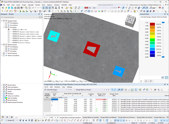
Do you have individual column sections and angled wall geometries, and need punching shear design for them?
No problem. In RFEM 6, you can perform punching shear design not only for rectangular and circular sections, but for any cross-section shape.
- Design of five types of seismic force-resisting systems (SFRS) includes Special Moment Frame (SMF), Intermediate Moment Frame (IMF), Ordinary Moment Frame (OMF), Ordinary Concentrically Braced Frame (OCBF), and Special Concentrically Braced Frame (SCBF)
- Ductility check of the width-to thickness ratios for webs and flanges
- Calculation of the required strength and stiffness for stability bracing of beams
- Calculation of the maximum spacing for stability bracing of beams
- Calculation of the required strength at hinge locations for stability bracing of beams
- Calculation of the column required strength with the option to neglect all bending moments, shear, and torsion for overstrength limit state
- Design check of column and brace slenderness ratios
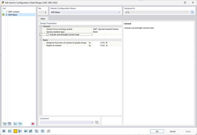
The relevant input for the design is defined in the Seismic Configuration. Afterwards, a new Seismic Configuration can be defined by entering a descriptive configuration name, and then selecting the applicable SFRS frame type and member type.
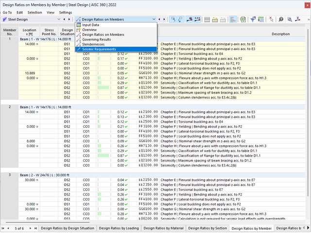
The seismic design result is categorized into two sections: member requirements and connection requirements.
The "Seismic Requirements" include the Required Flexural Strength and the Required Shear Strength of the beam-to-column connection for moment frames. They are listed in the ‘Moment Frame Connection by Member’ tab. For braced frames, the Required Connection Tensile Strength and the Required Connection Compressive Strength of the brace are listed in the ‘Brace Connection by Member’ tab.
The program provides the performed design checks in tables. The design check details clearly display the formulas and references to the standard.
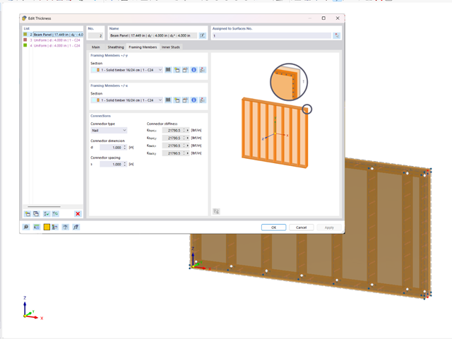
Using the "Beam Panel" thickness type, you can model timber panel elements in 3D space. You just specify the surface geometry and the timber panel elements are generated using an internal member-surface construct, including the simulation of the connection flexibility.
A "beam panel" provides you with the following advantages:
- Single-sided and double-sided sheathing is possible
- Automatic calculation of a semi-rigid coupling
- Boarded sheathing
- Stapled sheathing
- User-defined sheathing
- Representation as a complete geometric 3D object (frame, crosstie, column, sheeting, staples), including eccentricity
- Considering openings via surface cells
- Design of the structural elements utilizing the Timber Design add-on
- Independent of material (for example, drywall with cold-formed sections and gypsum fibreboards as the sheathing)
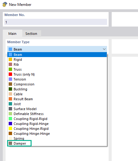
Using the "Damper" member type, you can define a damping coefficient, a spring constant, and a mass. This member type extends the possibilities within the Time History Analysis.
With regard to viscoelasticity, the "Damper" member type is similar to the Kelvin-Voigt model, which consists of the damping element and an elastic spring (both connected in parallel).

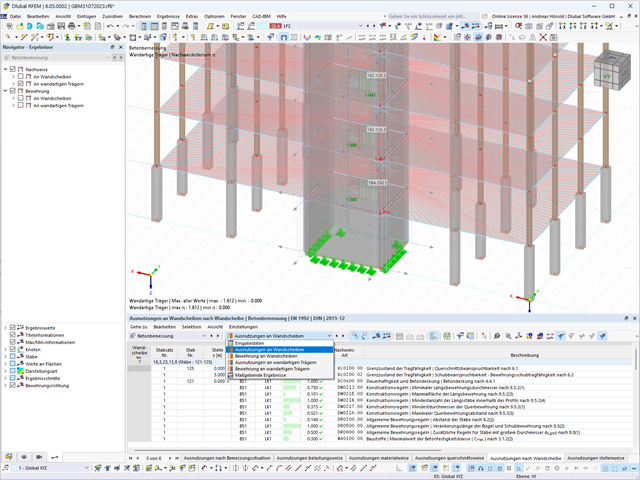
The building model is calculated in two phases:
- Global 3D calculation of the global model, where the slabs are modeled as a rigid plane (diaphragm) or as a bending plate
- Local 2D calculation of the individual floors
After the calculation, the results of the columns and walls from the 3D calculation and the results of the slabs from the 2D calculation are combined in a single model. This means that there is no need to switch between the 3D model and the individual 2D models of the slabs. The user only works with one model, saves valuable time, and avoids possible errors in the manual data exchange between the 3D model and the individual 2D ceiling models.
The vertical surfaces in the model can be divided into shear walls and opening lintels. The program automatically generates internal result members from these wall objects, so they can be designed as members according to any standard in the Concrete Design add-on.
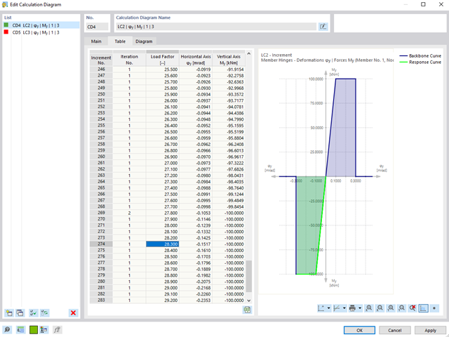
For calculation diagrams, you can use the "2D | Hinge" diagram type. These hinge diagrams show the hinge response of load situations for nonlinear hinges.
For calculations with several load situations, such as the case with the pushover analysis and time history analysis, you can evaluate the hinge condition in each load step.
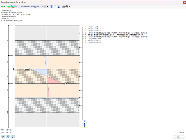
You have the option to perform the fire resistance design of surfaces using the reduced cross-section method. The reduction is applied over the surface thickness. It is possible to perform the design checks for all timber materials allowed for the design.
For cross-laminated timber, depending on the type of adhesive, you can select whether it is possible for individual carbonized layer parts to fall off, and whether you can expect increased charring in certain layer areas.
Shear walls and deep beams of a building model are available as independent objects in the design add-ons. This allows for faster filtering of the objects in results, as well as better documentation in the printout report.

In the Modal Analysis add-on, you have the option to automatically increase the sought eigenvalues until reaching a defined effective modal mass factor. All translational directions activated as masses for the modal analysis are taken into account.
Thus, it is possible to easily calculate the required 90% of the effective modal mass for the response spectrum method.
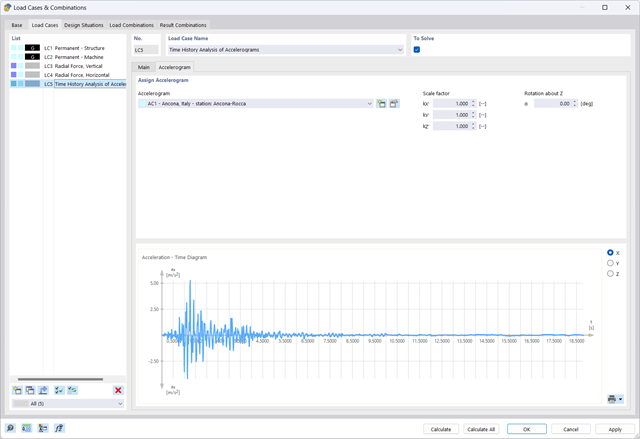
The Time History Analysis add-on provides you with accelerograms for the calculation. This extension allows for dynamic structural analysis of the acceleration-time diagrams.
There is an extensive library of earthquake records available for you, but you can also enter or import your own diagrams. The time history analysis is performed using the modal analysis or the linear implicit Newmark analysis.
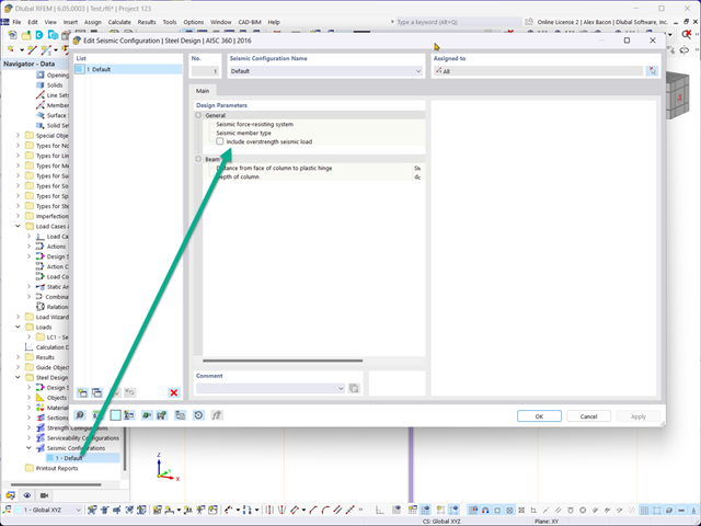
In the Concrete Design provides an option to perform seismic design according to AISC 341-16 for steel members.
Five SFRS types (Seismic Force-Resisting Systems) are available for this.
More Information
For a response spectrum analysis of building models, you can display the sensitivity coefficients for the horizontal directions by story.
These key figures allow you to interpret the sensitivity to stability effects.

The modal relevance factor (MRF) can help you to assess to which extent specific elements participate in a specific mode shape. The calculation is based on the relative elastic deformation energy of each individual member.
The MRF can be used to distinguish between local and global mode shapes. If multiple individual members show significant MRF (for example, > 20%), the instability of the entire structure or a substructure is very likely. On the other hand, if the sum of all MRFs for an eigenmode is around 100%, a local stability phenomenon (for example, buckling of a single bar) can be expected.
Furthermore, the MRF can be used to determine critical loads and equivalent buckling lengths of certain members (for example, for stability design). Mode shapes for which a specific member has small MRF values (for example, < 20%) can be neglected in this context.
The MRF is displayed by mode shape in the result table under Stability Analysis → Results by Members → Effective Lengths and Critical Loads.
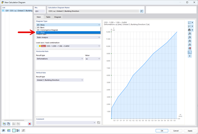
The "2D | Story" calculation diagram type is used to create result diagrams via the building axis. This allows you to easily analyze the behavior of the entire building under static and dynamic effects.
You can use this diagram type, for example, to visualize the seismic force over the building height.
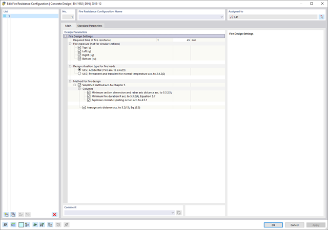
The Concrete Design add-on provides you with the option to perform the simplified fire resistance design according to EN 1992‑1‑2 for columns (Section 5.3.2) and beams (Section 5.6).
The following design checks are available for the simplified fire resistance design:
- Columns: Minimum cross-sectional dimensions for rectangular and circular sections according to Table 5.2a as well as Equation 5.7 for calculating time of fire exposure
- Beams: Minimum dimensions and center distances according to Table 5.5 and Table 5.6
You can determine the internal forces for the fire resistance design according to two methods.
- 1 Here, the internal forces of the accidental design situation are included directly into the design.
- 2 The internal forces of the design at normal temperature are reduced by the factor Eta,fi (ηfi), then used in the fire resistance design.
Furthermore, it is possible to modify the axis distance according to Eq. 5.5.
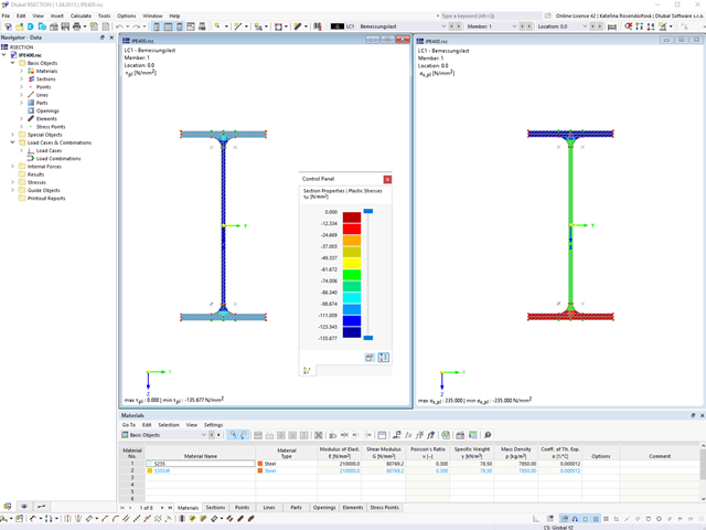
Within the "Plastic capacity design | Simplex Method" in RSECTION, the simultaneous variation of shear stresses over the cross-sectional area is performed in addition to the variation of axial stresses. This extended form of analysis allows you to use redistribution reserves, especially for the cross-sections subjected to shear loading, thus loading the cross-sections even more efficiently.
Go to Explanatory Video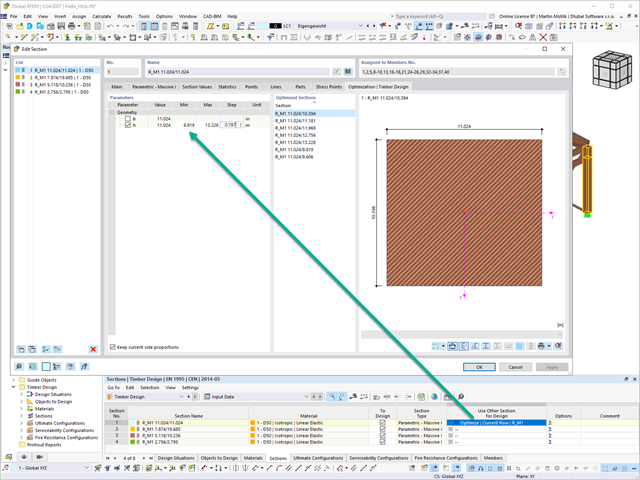
In the design add-ons (such as Steel Design, Timber Design, and so on), you can optimize cross-sections.
The optimization can be performed, for example, for standard cross-sections of a series, or for the width, height, and so on, in the case of parametric cross-sections.
Go to Explanatory Video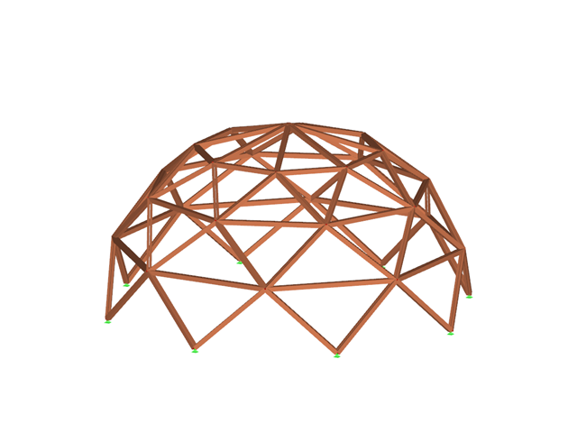
The Timber Design add-on for RFEM 6 / RSTAB 9 is multi-purpose and combines a large number of additional elements. [*S16332764*] Timber Design Add-on for RFEM 6
- Analysis of time diagrams and accelerograms (acceleration-time diagrams exciting the supports of a structure)
- Combination of user-defined time diagrams with nodal, member, and surface loads, as well as free and generated loads
- Combination of several independent excitation functions
- Linear implicit Newmark analysis or modal analysis in time history
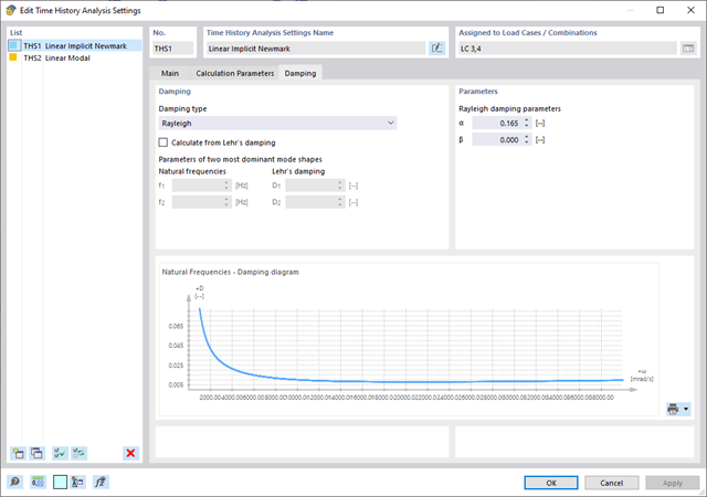
- Structural damping using Raleigh damping coefficients or Lehr's damping value
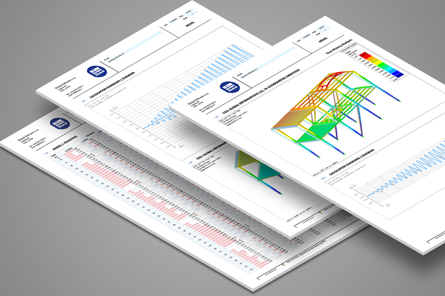
- Graphical display of results in calculation diagrams
- Result display in individual time steps or as an envelope during the entire time period
- Extensive library of seismic events (accelerograms)
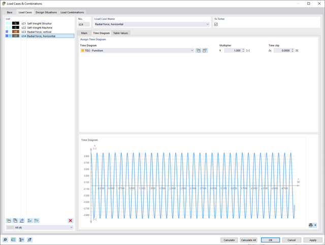
It is necessary to enter the required force-time diagrams. They can be combined in load cases or load combinations of the type Time History Analysis | Time Diagrams with the loading in order to define where and in which direction the force-time diagrams act.
The second option is to enter acceleration-time diagrams, which can be used in the load cases of the Time History Analysis | Accelerogram type.
All calculation parameters are specified in the time history analysis settings. These include, for example, the type of analysis method and the maximum calculation time.
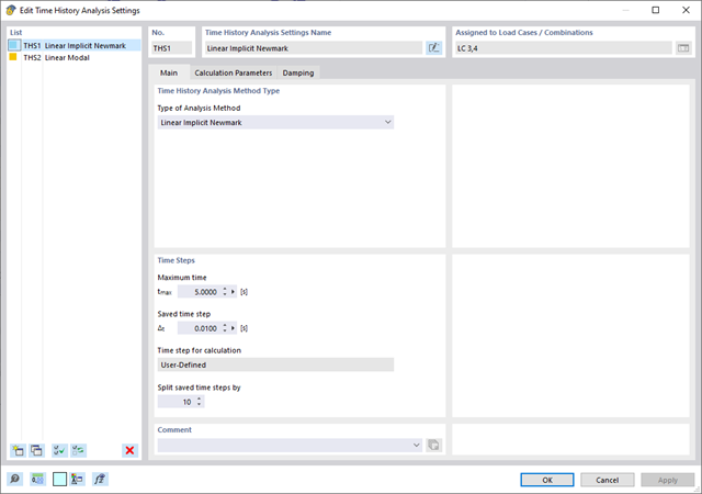
The time history analysis is performed with the modal analysis or the linear implicit Newmark analysis. The time history analysis in this add-on is limited to linear structural systems. Although the modal analysis represents a fast algorithm, it is necessary to use a certain number of eigenvalues to ensure the required accuracy of results.
The implicit Newmark analysis is a very precise method, independent of the number of eigenvalues used, but requires sufficient small time steps for the calculation.