9 Wyniki
Wyświetl wyniki:
Sortuj według:
- 002089
- Ogólne informacje
- Skręcanie skrępowane (7 stopni swobody) RFEM 6
- Skręcanie skrępowane (7 stopni swobody) RSTAB 9
- Uwzględnienie 7 lokalnych kierunków deformacji (ux , uy, uz, φx, φy, φz, ω ) lub 8 sił wewnętrznych (N , Vu, Vv, Mt, pri, Mt, s, Mu, Mv, Mω ) przy obliczaniu elementów prętowych
- Możliwość stosowania w połączeniu z analizą statyczno-wytrzymałościową według teorii II rzędu, i analiza dużych deformacji (można również uwzględnić imperfekcje)
- W połączeniu z rozszerzeniem Analiza stateczności umożliwia definiowanie współczynników obciążenia krytycznego i kształtów drgań dla problemów stateczności, takich jak wyboczenie skrętne i zwichrzenie
- Uwzględnianie blach czołowych i usztywnień poprzecznych jako sprężystości skrępowanej podczas obliczania przekrojów dwuteowych z automatycznym określaniem i wyświetlaniem graficznym sztywności sprężystości deplanacyjnej
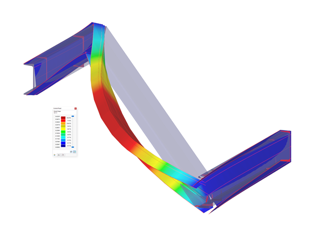
- Graficzne przedstawienie deplanacji przekroju prętów w stanie odkształcenia
- Pełna integracja z RFEM i RSTAB

- 002090
- Ogólne informacje
- Skręcanie skrępowane (7 stopni swobody) RFEM 6
- Skręcanie skrępowane (7 stopni swobody) RSTAB 9
Obliczenia skręcania skrępowanego można przeprowadzić dla całego układu. Uwzględniasz zatem dodatkową wartość 7 stopnia swobody w obliczeniach pręta. Sztywności połączonych elementów konstrukcyjnych są uwzględniane automatycznie. Oznacza to, że nie ma potrzeby' definiowania równoważnych sztywności sprężystych ani warunków podparcia dla układu odłączanego.
Następnie można wykorzystać siły wewnętrzne z obliczeń ze skręcaniem skrępowanym w rozszerzeniu do obliczeń. W zależności od materiału i wybranej normy należy uwzględnić bimoment wyboczeniowy i drugorzędny moment skręcający. Typowym zastosowaniem jest analiza stateczności według teorii drugiego rzędu z wykorzystaniem imperfekcji w konstrukcjach stalowych.
Czy wiecie, że...? Zastosowanie nie ogranicza się do przekrojów stalowych cienkościennych. Pozwala to na przykład na przeprowadzenie obliczeń idealnego momentu krytycznego dla belek o przekrojach z drewna litego.
- 002401
- Ogólne informacje
- Skręcanie skrępowane (7 stopni swobody) RFEM 6
- Skręcanie skrępowane (7 stopni swobody) RSTAB 9
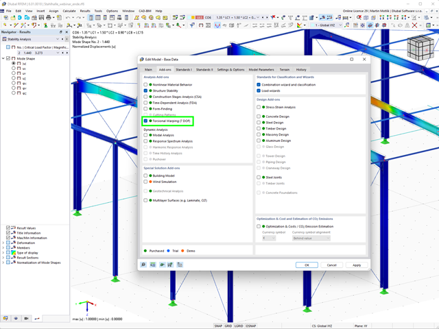
- Funkcję skręcania skrępowanego można aktywować lub dezaktywować w zakładce Rozszerzenia w Danych podstawowych modelu.
- Po aktywowaniu rozszerzenia interfejs użytkownika w programie RFEM zostaje rozszerzony o nowe wpisy w nawigatorze, tabelach i oknach dialogowych.
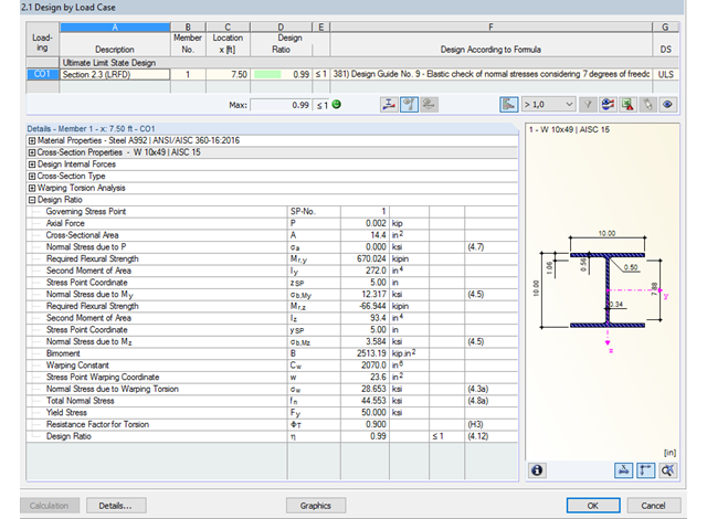
Dzięki zintegrowanemu rozszerzeniu modułu RF-/STEEL Warping Torsion, możliwe jest przeprowadzenie obliczeń zgodnie z Design Guide 9 w RF-/STEEL AISC.
Obliczenia są przeprowadzane z 7 stopniami swobody zgodnie z teorią skręcania skrępowanego i umożliwiają realistyczne obliczenia stateczności z uwzględnieniem skręcania.
Definiowanie krytycznego momentu wyboczeniowego odbywa się w module RF-/STEEL AISC za pomocą solwera wartości własnych, który umożliwia dokładne określenie krytycznego obciążenia wyboczeniowego.
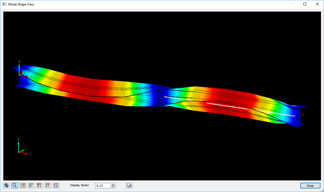
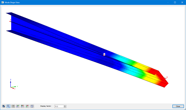
Solwer wartości własnych pokazuje okno z grafiką wartości własnych, które umożliwia sprawdzenie warunków brzegowych.
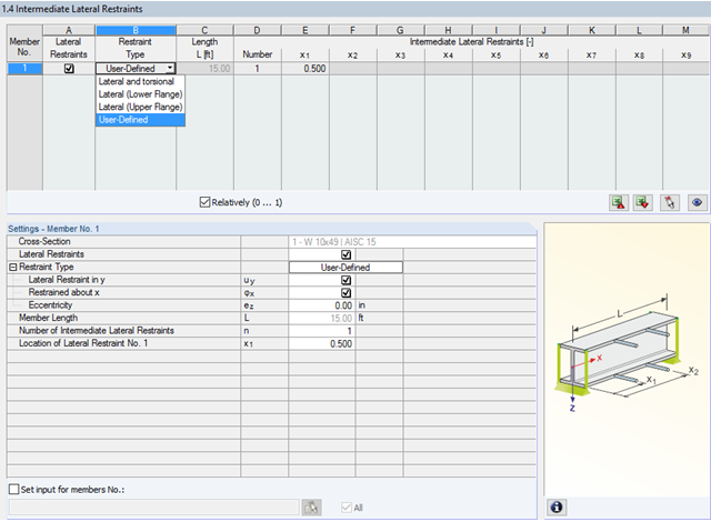
W programie STEEL AISC możliwe jest uwzględnienie pośrednich podpór bocznych w dowolnym miejscu. Na przykład, możliwa jest stabilizacja tylko górnej półki.
Ponadto można przypisać boczne podpory pośrednie zdefiniowane przez użytkownika; na przykład pojedyncze sprężyny obrotowe i sprężyny translacyjne w dowolnym miejscu przekroju.
- Stosuje się do prętów zdefiniowanych jako zbiory prętów
- Oddzielny solwer uwzględniający 7 kierunków deformacji (ux , uy, uz, φx, φy, φz, ω ) lub 8 sił wewnętrznych (N, Vu, Vv, Mt, pri, Mt, s, Mu, Mv,M )
- Projektowanie nieliniowe według analizy drugiego rzędu
- Wprowadzanie imperfekcji
- Obliczanie współczynników obciążenia krytycznego i postaci wyboczenia oraz ich wizualizacja (wraz z skręcaniem skrępowanym)
- Integracja z wymiarowaniem prętów w modułach dodatkowych RF-/STEEL AISC i RF-/STEEL EC3
- Dostępne dla wszystkich przekrojów stalowych cienkościennych
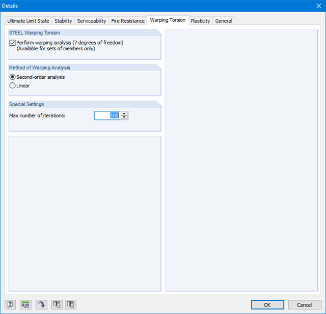
Ponieważ moduł RF-/STEEL Warping Torsion jest w pełni zintegrowany z modułami RF-/STEEL AISC i RF‑/STEEL EC3, dane są wprowadzane w taki sam sposób, jak w przypadku obliczeń w tych modułach. W oknie dialogowym Szczegóły, zakładka Skręcanie skrępowane (patrz rysunek po prawej stronie), konieczne jest tylko zaznaczenie opcji "Przeprowadzić analizę skręcania skrępowanego". W tym oknie dialogowym można również zdefiniować maksymalną liczbę iteracji.
Analiza skręcania skrępowanego jest przeprowadzana dla zbiorów prętów w modułach RF-/STEEL AISC i RF-/STEEL EC3. Można dla nich zdefiniować warunki brzegowe, takie jak podpory węzłowe lub zwolnienia na końcach prętów.
Możliwe jest również określenie imperfekcji do obliczeń nieliniowych.
Wyniki analizy skręcania skrępowanego są wyświetlane w modułach RF-/STEEL AISC i RF-/STEEL EC3 w zwykły sposób. Odpowiednie okna wyników zawierają między innymi wartości krytycznego skręcania i skręcania, siły wewnętrzne oraz podsumowanie obliczeń.
Graficzne przedstawienie postaci drgań (wraz z deplanacją) umożliwia realistyczną ocenę zachowania się wyboczenia.