81 Wyniki
Wyświetl wyniki:
Sortuj według:
- 002074
- Ogólne informacje
- Analiza stateczności konstrukcji RFEM 6
- Analiza stateczności konstrukcji RSTAB 9
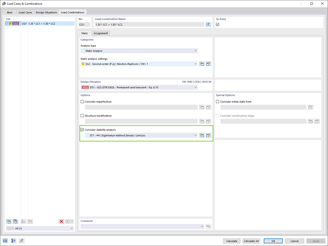
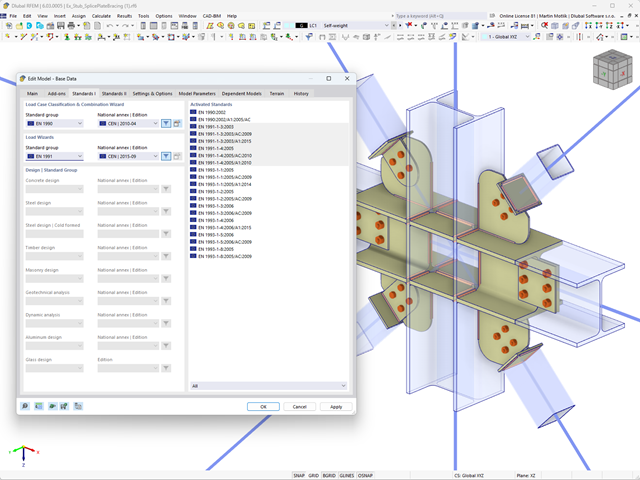
Jeżeli w programie istnieje przypadek obciążenia lub kombinacja obciążeń, obliczenia stateczności są aktywowane. Można zdefiniować inny przypadek obciążenia, na przykład w celu uwzględnienia naprężenia początkowego.
W tym celu należy określić, czy ma zostać przeprowadzona analiza liniowa czy nieliniowa. W zależności od przypadku zastosowania, można wybrać bezpośrednią metodę obliczeniową, taką jak metoda Lanczosa lub metoda iteracji ICG. Pręty niezintegrowane z powierzchniami są zazwyczaj wyświetlane jako elementy prętowe z dwoma węzłami ES. W przypadku zastosowania takich elementów program nie może określić wyboczenia lokalnego pojedynczych prętów. Z tego względu'istnieje możliwość automatycznego dzielenia prętów.
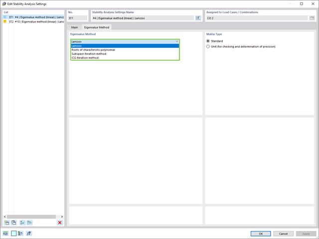
W przypadku analizy wartości własnych dostępnych jest kilka metod:
- Metody bezpośrednie
- Metody bezpośrednie (Lanczosa [RFEM], pierwiastki z wielomianu charakterystycznego [RFEM], metoda iteracji podprzestrzeni [RFEM/RSTAB], przesunięta iteracja odwrócona [RSTAB]) są odpowiednie dla małych i średnich modeli. Z szybkich metod rozwiązywania problemów należy korzystać tylko w przypadku, gdy komputer posiada dużą ilość pamięci RAM.
- Metoda iteracji ICG (niekompletny sprzężony gradient [RFEM])
- Z drugiej strony, ta metoda wymaga tylko niewielkiej ilości pamięci. Wartości własne są określane jedna po drugiej. Może być stosowany do obliczania dużych układów konstrukcyjnych o niewielkiej liczbie wartości własnych.
Rozszerzenie Stateczność konstrukcji umożliwia nieliniową analizę stateczności przy użyciu metody przyrostowej. Analiza ta dostarcza wyniki zbliżone do rzeczywistości również w przypadku konstrukcji nieliniowych. Współczynnik obciążenia krytycznego jest określany poprzez stopniowe zwiększanie obciążeń w podstawowym przypadku obciążenia, aż do osiągnięcia niestateczności. Przyrost obciążenia uwzględnia nieliniowości, takie jak ulegające uszkodzeniu pręty, podpory i fundamenty oraz nieliniowości materiałowe. Po zwiększeniu obciążenia można opcjonalnie przeprowadzić liniową analizę stateczności na ostatnim stabilnym stanie w celu określenia postaci stateczności.
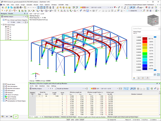
Jako pierwsze wyniki program przedstawia współczynniki obciążenia krytycznego. Następnie można przeprowadzić ocenę zagrożeń stateczności. W przypadku modeli prętowych w tabelach wyświetlane są wynikowe długości efektywne i obciążenia krytyczne prętów.
W następnym oknie wyników można sprawdzić znormalizowane wartości własne posortowane według węzła, pręta i powierzchni. Grafika wartości własnych umożliwia ocenę zachowania wyboczeniowego. Ułatwia to podjęcie środków zaradczych.
- 002073
- Ogólne informacje
- Analiza stateczności konstrukcji RFEM 6
- Analiza stateczności konstrukcji RSTAB 9
- Obliczanie modeli składających się z elementów prętowych, powłokowych i bryłowych
- Nieliniowa analiza stateczności
- Możliwość uwzględniania sił osiowych od wstępnego sprężenia
- Cztery dostępne solvery do rozwiązywania równań dla efektywnego obliczania różnych modeli konstrukcyjnych
- Opcjonalne uwzględnianie zmian w sztywności w programie RFEM/RSTAB
- Wyszukiwanie postaci wyboczeniowych o krytycznym mnożniku obciążenia większym niż zadany przez użytkownika (metoda "przesunięcia")
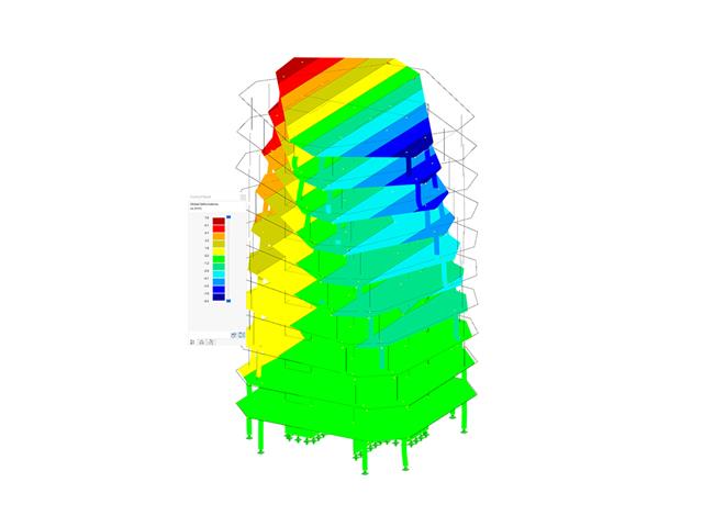
- Możliwość określania wektorów własnych dla modeli niestatecznych (w celu zidentyfikowania przyczyny niestateczności)
- Wizualizacja postaci niestateczności
- Podstawa określania imperfekcji
- 002111
- Ogólne informacje
- Analiza naprężeniowo-odkształceniowa RFEM 6
- Analiza naprężeniowo-odkształceniowa RSTAB 9
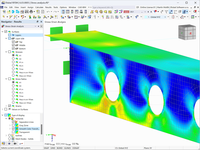
- Ogólna analiza naprężeniowa
- Automatyczny import sił wewnętrznych z programu RFEM/RSTAB
- Graficzne i numeryczne przedstawianie naprężeń, odkształceń, luzu i stopni wykorzystania w pełni zintegrowane z RFEM/RSTAB
- Zdefiniowana przez użytkownika specyfikacja naprężenia granicznego
- Podsumowanie podobnych elementów konstrukcyjnych do obliczeń
- Szeroki zakres opcji umożliwiających dostosowywania sposobu wyświetlania wyników
- Przejrzyste tabele wyników dla szybkiego ich przeglądania po zakończeniu obliczeń
- Łatwa możliwość identyfikacji wyników dzięki w pełni udokumentowanej metodzie obliczeniowej wraz ze wszystkimi wzorami
- Wysoka wydajność pracy dzięki minimalnej ilości danych wejściowych
- Elastyczność dzięki szczegółowym opcjom ustawień dla podstawy i zakresu obliczeń
- Wyświetlanie szarej strefy dla nieistotnych zakresów wartości: Funkcja produktu "Analiza naprężeniowo-odkształceniowa z wyświetlaniem w szarej strefie"
- 002112
- Ogólne informacje
- Analiza naprężeniowo-odkształceniowa RFEM 6
- Analiza naprężeniowo-odkształceniowa RSTAB 9
- Optymalizacja przekroju
- Transfer zoptymalizowanych przekrojów do RFEM/RSTAB
- Wymiarowanie dowolnego przekroju cienkościennego z RSECTION
- Odwzorowanie wykresu naprężeń na przekroju
- Wyznaczanie naprężeń normalnych, ścinających i równoważnych
- Wyświetlanie składowych naprężeń dla poszczególnych typów sił wewnętrznych pręta
- Szczegółowe przedstawienie naprężeń we wszystkich punktach naprężeniowych
- Wyznaczanie największego Δσ dla każdego punktu naprężenia (na przykład do obliczeń zmęczenia)
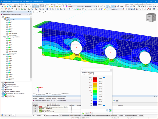
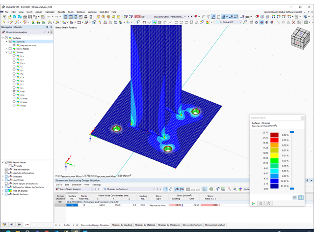
- Wyświetlanie w kolorze naprężeń i stopni wykorzystania w celu szybkiego przeglądu stref krytycznych lub przewymiarowanych
- Wyświetlanie wykazów materiałów
- Wyznaczanie naprężeń głównych i podstawowych, naprężeń membranowych i stycznych oraz naprężeń zastępczych i zastępczych naprężeń membranowych
- Analiza naprężeń dla elementów konstrukcyjnych o dowolnym kształcie
- Obliczanie naprężeń zastępczych według różnych metod:
- Hipoteza energii odkształcenia (von Mises)
- Schubspannungshypothese (Tresca)
- Normalspannungshypothese (Rankine)
- Hauptdehnungshypothese (Bach)
- Możliwość optymalizacji grubości powierzchni i transferu danych do programu RFEM
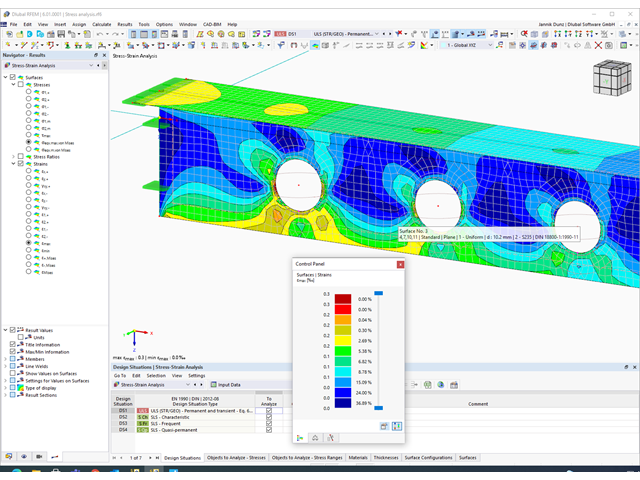
- Ausgabe der Dehnungen
- Szczegółowe wyniki dla różnych składników naprężeń i stopni wykorzystania w tabelach i w grafice
- Filtermöglichkeit für Volumenkörper, Flächen, Linien und Knoten in Tabellen
- Querschubspannungen nach Mindlin, Kirchhoff oder freier Eingabe
- Spannungsauswertung für Schweißnähte an Verbindungslinien zwischen Flächen: Przejdź do funkcji produktu "Spoina liniowa"
- 002115
- Wyniki
- Analiza naprężeniowo-odkształceniowa RFEM 6
- Analiza naprężeniowo-odkształceniowa RSTAB 9
Po zakończeniu obliczeń wyniki są uporządkowane w sposób przejrzysty. W ten sposób program wyświetla maksymalne naprężenia i stopnie naprężeń posortowane według przekroju, pręta/powierzchni, bryły, zbioru prętów, położenia x itd. Oprócz wartości wyników w formie tabelarycznej rozszerzenie wyświetla również odpowiednią grafikę przekroju z punktami naprężeniowymi, wykresem naprężeń i wartościami. Stopień wykorzystania można odnieść do dowolnego rodzaju naprężenia. Aktualnie wybrana lokalizacja na elemencie zostanie wyróżniona na modelu analitycznym w programie RFEM/RSTAB.
Oprócz oceny tabelarycznej program oferuje jeszcze więcej. Naprężenia i stopnie wykorzystania można również sprawdzić graficznie na modelu w programie RFEM/RSTAB. Istnieje możliwość indywidualnego dostosowania kolorów i wartości.
Wyświetlanie wykresów wyników dla pręta lub zbioru prętów umożliwia dokładną ocenę. Dla każdego miejsca obliczeniowego można otworzyć odpowiednie okno dialogowe, w którym można sprawdzić odpowiednie do obliczeń właściwości przekroju i składowe naprężeń w dowolnym punkcie naprężeniowym. Na koniec istnieje możliwość wydrukowania odpowiedniej grafiki wraz ze wszystkimi szczegółami obliczeń.
Parametry załączników krajowych (NA) do Eurokodu 3 z następujących krajów są zintegrowane:
-
 DIN EN 1993-1-1/NA:2016-04 (Niemcy)
 -
 ÖNORM EN 1993-1-1/NA:2015-12 (Austria)
 -
 SN EN 1993-1-1/NA:2016-07 (Szwajcaria)
 -
 BDS EN 1993-1-1/NA:2015-10 (Bułgaria)
 -
 BS EN 1993-1-1/NA:2016-07 (Wielka Brytania)
 -
 CEN EN 1993-1-1/2015-06 (Unia Europejska)
 -
 CYS EN 1993-1-1/NA:2015-07 (Cypr)
 -
 CSN EN 1993-1-1/NA:2016-06 (Republika Czeska)
 -
 DS EN 1993-1-1/NA:2015-07 (Dania)
 -
 ELOT EN 1993-1-1/NA:2017-01 (Grecja)
 -
 EVS EN 1993-1-1/NA:2015-08 (Estonia)
 -
 HRN EN 1993-1-1/NA:2016-03 (Chorwacja)
 -
 I S. EN 1993-1-1/NA:2016-03 (Irlandia)
 -
 ILNAS EN 1993-1-1/NA:2015-06 (Luksemburg)
 -
 IST EN 1993-1-1/NA:2015-11 (Islandia)
 -
 LST EN 1993-1-1/NA:2017-01 (Litwa)
 -
 LVS EN 1993-1-1/NA:2015-10 (Łotwa)
 -
 MS EN 1993-1-1/NA:2010-01 (Malezja)
 -
 MSZ EN 1993-1-1/NA:2015-11 (Węgry)
 -
 NBN EN 1993-1-1/NA:2015-07 (Belgia)
 -
 NEN EN 1993-1-1/NA:2016-12 (Holandia)
 -
 NF EN 1993-1-1/NA:2016-02 (Francja)
 -
 NP EN 1993-1-1/NA:2009-03 (Portugalia)
 -
 NS EN 1993-1-1/NA:2015-09 (Norwegia)
 -
 PN EN 1993-1-1/NA:2015-08 (Polska)
 -
 SFS EN 1993-1-1/NA:2015-08 (Finlandia)
 -
 SIST EN 1993-1-1/NA:2016-09 (Słowenia)
 -
 SR EN 1993-1-1/NA:2016-04 (Rumunia)
 -
 SS EN 1993-1-1/NA:2019-05 (Singapur)
 -
 SS EN 1993-1-1/NA:2015-06 (Szwecja)
 -
 STN EN 1993-1-1/NA:2015-10 (Słowacja)
 -
 TKP EN 1993-1-1/NA:2015-04 (Białoruś)
 -
 UNE EN 1993-1-1/NA:2016-02 (Hiszpania)
 -
 UNI EN 1993-1-1/NA:2015-08 (Włochy)
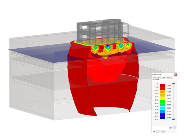
- Realistyczne odwzorowanie interakcji między budynkiem a gruntem
- Realistyczne odwzorowanie oddziaływania poszczególnych fundamentów na siebie nawzajem
- Biblioteka parametrów gruntowych z możliwością rozszerzania
- Możliwość uwzględniania wielu próbek gruntu z różnych lokalizacji, także poza obrysem budynku
- Określanie osiadań oraz wykresów naprężeń w gruncie oraz ich prezentacja w formie graficznej i tabelarycznej