71 Wyniki
Wyświetl wyniki:
Sortuj według:
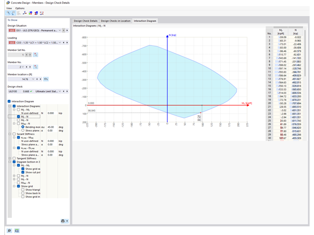
Czy wiesz, że wykresy interakcji moment-siła (wykresy MN) można wyświetlić również graficznie? Umożliwia to wyświetlenie nośności przekroju w przypadku interakcji momentu zginającego i siły osiowej. Oprócz wykresów interakcji związanych z osiami przekroju (wykres My-N i wykres Mz-N) można również wygenerować indywidualny wektor momentów w celu utworzenia wykresu interakcji Mres -N. Płaszczyznę przekroju wykresów MN można wyświetlić na wykresie interakcji 3D.Program wyświetla odpowiednie pary wartości stanu granicznego nośności w tabeli. Tabela jest dynamicznie powiązana z wykresem, dzięki czemu wybrany punkt graniczny jest również wyświetlany na wykresie.
- 002469
- Ogólne informacje
- Projektowanie konstrukcji betonowych RFEM 6
- Projektowanie konstrukcji betonowych RSTAB 9
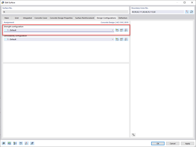
Pracujesz z elementami konstrukcyjnymi składającymi się z płyt? W takim przypadku należy przeprowadzić obliczenia na ścinanie z uwzględnieniem wymagań obliczania przebicia, na przykład zgodnie z 6.4, EN 1992-1-1. Oprócz płyt stropowych można w ten sposób wymiarować również płyty fundamentowe.
W konfiguracji stanu granicznego nośności dla wymiarowania betonu można zdefiniować parametry obliczeń przebicia dla wybranych węzłów.
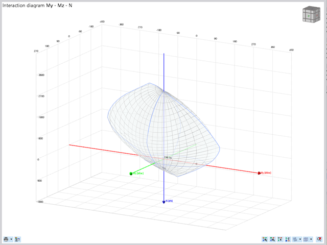
Projektowanie konstrukcji betonowych | Wykres interakcji My-Mz-N (3D) przekrojów z betonu zbrojonego
Na pytanie 'Ile można przewozić?' zazwyczaj odpowiada 'Tak'. Do graficznego przedstawiania stanu granicznego nośności przekrojów żelbetowych wymagany jest trójwymiarowy wykres interakcji momentu-momentu-siła osiowa. Oprogramowanie do analizy statyczno-wytrzymałościowej firmy Dlubal właśnie to oferuje.
Dzięki dodatkowemu wyświetleniu oddziaływania obciążenia można łatwo rozpoznać lub zwizualizować przekroczenie granicznej nośności przekroju żelbetowego. Ponieważ możesz kontrolować właściwości wykresu, możesz dostosować wygląd wykresu My-Mz-N do swoich potrzeb.
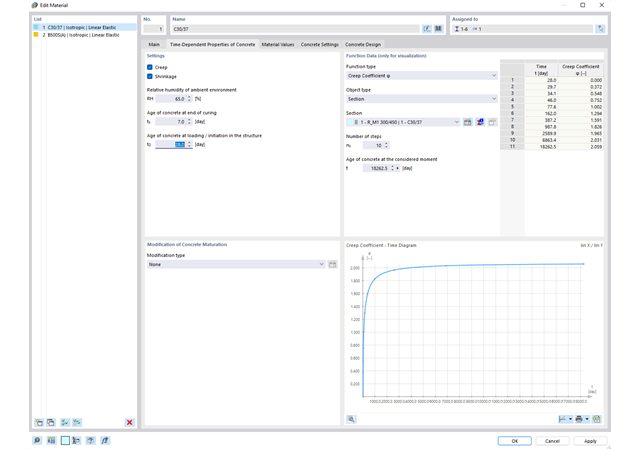
Właściwości betonu, zależne od czasu, takie jak pełzanie i skurcz, są bardzo ważne dla obliczeń. Można je zdefiniować bezpośrednio dla materiału w programie do analizy statyczno-wytrzymałościowej. W oknie dialogowym do wprowadzania danych wyświetlany jest przebieg czasowy funkcji pełzania lub skurczu. Można łatwo wybrać modyfikację zastosowanego wieku betonu, na przykład ze względu na obróbkę termiczną.
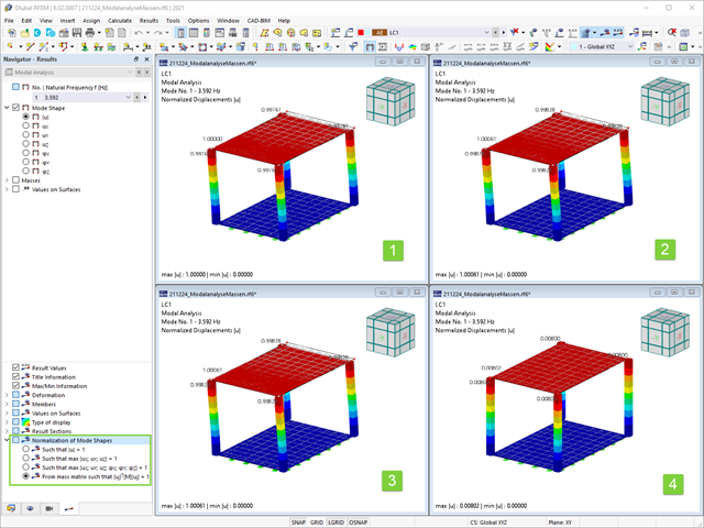
Jak już wiesz, po pomyślnym zakończeniu obliczeń wyniki przypadku obciążenia w Analizie modalnej są wyświetlane w programie. Die erste Eigenform ist für Sie also sofort grafisch oder animiert zu sehen. Dabei können Sie die Darstellung der Eigenformnormierung komfortabel anpassen. Erledigen Sie das am besten direkt im Ergebnisnavigator, wo Sie zur Visualisierung der Eigenformen eine von vier Optionen auswählen:
- Wert des Eigenformvektors uj auf 1 skalieren (berücksichtigt nur die Translationskomponenten)
- Auswahl der maximalen Translationskomponente des Eigenvektors und Einstellung auf 1
- Betrachtung der gesamten Eigenform (inklusive der Rotationskomponenten), Auswahl des Maximums und Einstellung auf 1
- Setzen der modalen Massen mi für jeden Eigenwert auf 1 kg
Ausführlichere Erläuterungen der Normierung der Eigenformen finden Sie hier: Instrukcja online .
Czy obliczenia się zakończyły? Wyniki analizy modalnej są wówczas dostępne zarówno w formie graficznej, jak i tabelarycznej. Wyświetl tabele wyników dla przypadku obciążenia lub przypadków obciążeń analizy modalnej. Dzięki temu na pierwszy rzut oka można zobaczyć wartości własne, częstotliwości kątowe, częstotliwości i okresy drgań własnych konstrukcji. W przejrzysty sposób wyświetlane są również efektywne masy modalne, modalne współczynniki masy i współczynniki udziału.
.png?mw=640&hash=5a991f211d984ac624978f514e70c53da263e5d9)
W zależności od siły osiowej N, można wygenerować linię krzywizny momentu dla dowolnego wektora momentu. Program pokazuje również pary wartości wyświetlanego wykresu w tabeli. Ponadto można aktywować jako dodatkowy wykres sieczny i sztywność styczną przekroju żelbetowego, należące do wykresu krzywizny momentu.
Odkształcenie prętów i powierzchni jest określane z uwzględnieniem zarysowanego (stan II) lub niezarysowanego (stan I) przekroju żelbetowego. Podczas określania sztywności można uwzględnić usztywnienie przy rozciąganiu między rysami, zwane 'usztywnieniem przy rozciąganiu', zgodnie z zastosowaną normą obliczeniową.

- 002090
- Ogólne informacje
- Skręcanie skrępowane (7 stopni swobody) RFEM 6
- Skręcanie skrępowane (7 stopni swobody) RSTAB 9
Obliczenia skręcania skrępowanego można przeprowadzić dla całego układu. Uwzględniasz zatem dodatkową wartość 7 stopnia swobody w obliczeniach pręta. Sztywności połączonych elementów konstrukcyjnych są uwzględniane automatycznie. Oznacza to, że nie ma potrzeby' definiowania równoważnych sztywności sprężystych ani warunków podparcia dla układu odłączanego.
Następnie można wykorzystać siły wewnętrzne z obliczeń ze skręcaniem skrępowanym w rozszerzeniu do obliczeń. W zależności od materiału i wybranej normy należy uwzględnić bimoment wyboczeniowy i drugorzędny moment skręcający. Typowym zastosowaniem jest analiza stateczności według teorii drugiego rzędu z wykorzystaniem imperfekcji w konstrukcjach stalowych.
Czy wiecie, że...? Zastosowanie nie ogranicza się do przekrojów stalowych cienkościennych. Pozwala to na przykład na przeprowadzenie obliczeń idealnego momentu krytycznego dla belek o przekrojach z drewna litego.
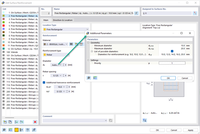
Istniejące zbrojenie powierzchniowe można automatycznie zaprojektować tak, aby pokryć wymagane zbrojenie. Można wybrać, czy automatycznie ma być definiowana średnica zbrojenia, czy też rozstaw prętów.
Przejdź do filmu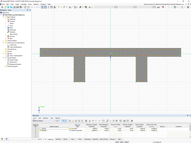
W rozszerzeniu Projektowanie konstrukcji betonowych można wymiarować dowolny przekrój RSECTION. Otulinę betonową, zbrojenie na ścinanie i zbrojenie podłużne definiuje się bezpośrednio w RSECTION.
Po zaimportowaniu przekroju ze zbrojeniem RSECTION do programu RFEM 6, można go również wykorzystać do obliczeń w rozszerzeniu Projektowanie konstrukcji betonowych.
Przejdź do filmu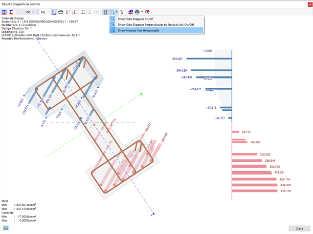
Istniejące naprężenia i odkształcenia przekroju betonowego i zbrojenia można wyświetlić w postaci obrazu naprężeń 3D lub grafiki 2D. W zależności od tego, które wyniki zostaną wybrane w drzewie wyników, naprężenia lub odkształcenia są wyświetlane w zdefiniowanym zbrojeniu podłużnym pod oddziaływaniami obciążeń lub granicznymi siłami wewnętrznymi.
- 002165
- Ogólne informacje
- Skręcanie skrępowane (7 stopni swobody) RFEM 6
- Skręcanie skrępowane (7 stopni swobody) RSTAB 9
W porównaniu z modułem dodatkowym RF-/STEEL Warping Torsion (RFEM 5/RSTAB 8) do rozszerzenia Skręcanie skrępowane (7 DOF) dla programu RFEM 6/RSTAB 9 dodano następujące nowe funkcje:
- Pełna integracja ze środowiskiem RFEM 6 i RSTAB 9
- Siódmy stopień swobody jest bezpośrednio uwzględniany w obliczeniach prętów w programie RFEM/RSTAB na całym układzie
- Nie ma już potrzeby definiowania warunków podparcia lub sztywności sprężystej do obliczeń w uproszczonym układzie zastępczym
- Możliwość łączenia z innymi rozszerzeniami, na przykład do obliczania obciążeń krytycznych dla wyboczenia skrętnego i zwichrzenia z analizą stateczności
- Brak ograniczeń dla stalowych przekrojów cienkościennych (możliwe jest również obliczenie momentu krytycznego, na przykład dla belek o masywnych przekrojach drewnianych)
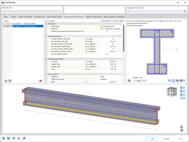
Zbrojenie na ścinanie i zbrojenie podłużne można zdefiniować indywidualnie dla każdego pręta. W tym przypadku dostępne są różne szablony do wprowadzania zbrojenia.
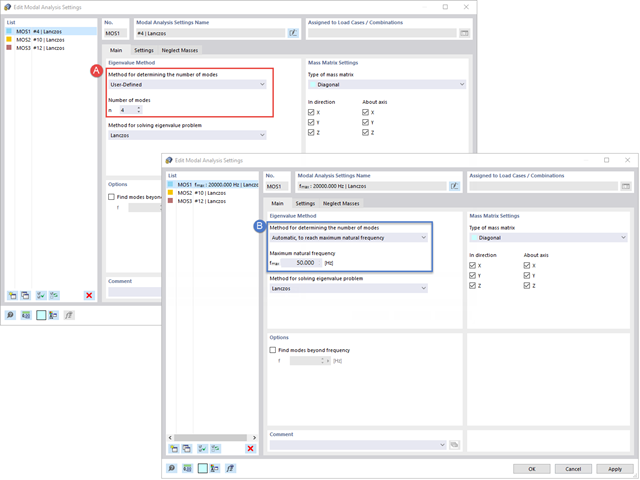
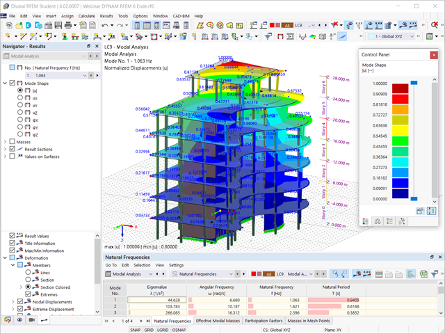
Twoim celem jest określenie liczby postaci drgań własnych? Program oferuje dwie metody. Z jednej strony, można ręcznie zdefiniować liczbę najmniejszych kształtów drgań, które mają zostać obliczone. W tym przypadku liczba dostępnych kształtów postaci zależy od stopni swobody (tzn. liczby punktów mas swobodnych pomnożonych przez liczbę kierunków, w których działają masy). Jest to jednak ograniczone do 9999. Z drugiej strony, maksymalną częstotliwość drgań własnych można ustawić w taki sposób, w jaki program określił kształty automatycznie, aż do osiągnięcia zadanej częstotliwości drgań własnych.
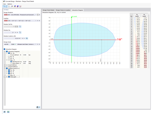
Czy chcesz określić nośność przekroju żelbetowego na zginanie dwukierunkowe? W tym celu należy najpierw aktywować wykres interakcji moment-moment (wykres My-Mz). Wykres My-Mz przedstawia poziomy przekrój przez trójwymiarowy wykres dla określonej siły osiowej N. Dzięki połączeniu z trójwymiarowym wykresem interakcji można tam również zwizualizować płaszczyznę przekroju.
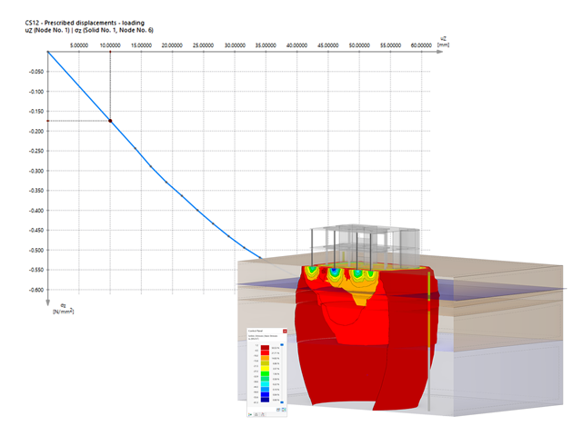
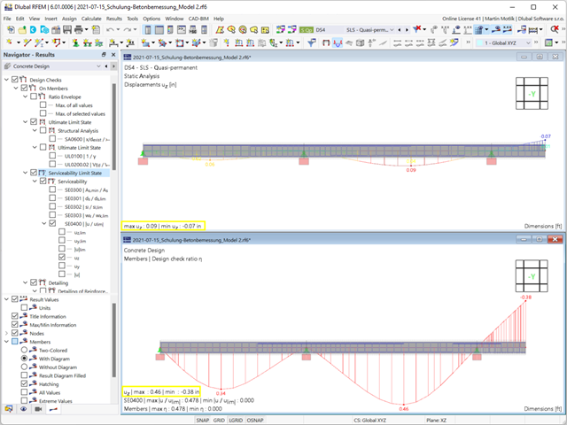
Czy jesteś gotowy na ocenę? Skorzystaj z wykresów obliczeniowych, które pokazują rozkład określonego wyniku podczas obliczeń.
Przypisanie osi pionowej i poziomej wykresu obliczeniowego można dowolnie definiować. Umożliwia to np. wyświetlenie przebiegu osiadania określonego węzła w zależności od obciążenia.
- 002089
- Ogólne informacje
- Skręcanie skrępowane (7 stopni swobody) RFEM 6
- Skręcanie skrępowane (7 stopni swobody) RSTAB 9
- Uwzględnienie 7 lokalnych kierunków deformacji (ux , uy, uz, φx, φy, φz, ω ) lub 8 sił wewnętrznych (N , Vu, Vv, Mt, pri, Mt, s, Mu, Mv, Mω ) przy obliczaniu elementów prętowych
- Możliwość stosowania w połączeniu z analizą statyczno-wytrzymałościową według teorii II rzędu, i analiza dużych deformacji (można również uwzględnić imperfekcje)
- W połączeniu z rozszerzeniem Analiza stateczności umożliwia definiowanie współczynników obciążenia krytycznego i kształtów drgań dla problemów stateczności, takich jak wyboczenie skrętne i zwichrzenie
- Uwzględnianie blach czołowych i usztywnień poprzecznych jako sprężystości skrępowanej podczas obliczania przekrojów dwuteowych z automatycznym określaniem i wyświetlaniem graficznym sztywności sprężystości deplanacyjnej
- Graficzne przedstawienie deplanacji przekroju prętów w stanie odkształcenia
- Pełna integracja z RFEM i RSTAB
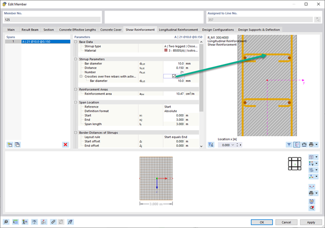
W zakładce "Zbrojenie na ścinanie" można wybrać opcję "Powiązania krzyżowe na wolnych prętach zbrojeniowych z aktywnym wyborem w oknie graficznym". Pozwala to na umieszczenie dodatkowych powiązań krzyżowych na wolnych prętach zbrojenia podłużnego.
Pozycję więzów krzyżowych można aktywować lub dezaktywować w infografice. Powiązania krzyżowe są uwzględniane podczas kontroli stanu granicznego nośności i obliczeń konstrukcji. Są one dostępne dla obliczeń zgodnie z EN 1992-1-1.
Przejdź do filmu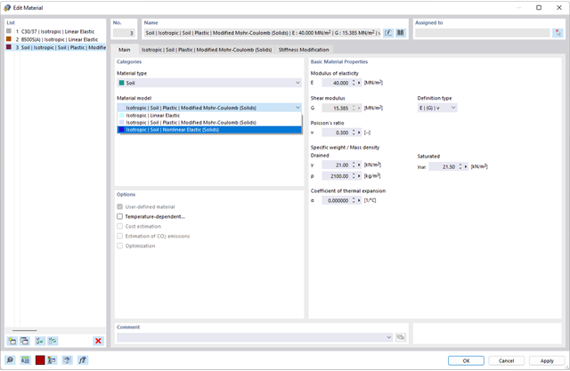
Czy chcesz modelować i analizować zachowanie bryły gruntowej? Aby to zapewnić, w programie RFEM zaimplementowano odpowiednie modele materiałowe.
Można użyć zmodyfikowanego modelu Mohra-Coulomba z liniowo-sprężystym modelem idealnie plastycznym lub nieliniowo sprężystym modelem z edometryczną relacją naprężenie-odkształcenie. Kryterium graniczne, które opisuje przejście od obszaru sprężystości do obszaru płynięcia plastycznego, jest zdefiniowane według Mohra-Coulomba.