AIJ Examples Case D - High-Rise Bilding in Center of Lower Buildings

Introduction

The Architectural Institute of Japan (AIJ) has presented a number of well-known benchmark scenarios of wind simulation.
The following article deals with "Case D - High-Rise Building Among City Blocks".
In the following, the described scenario is simulated in RWIND 2 and the results are compared with the simulated and experimental results by the AIJ.

Model Layout

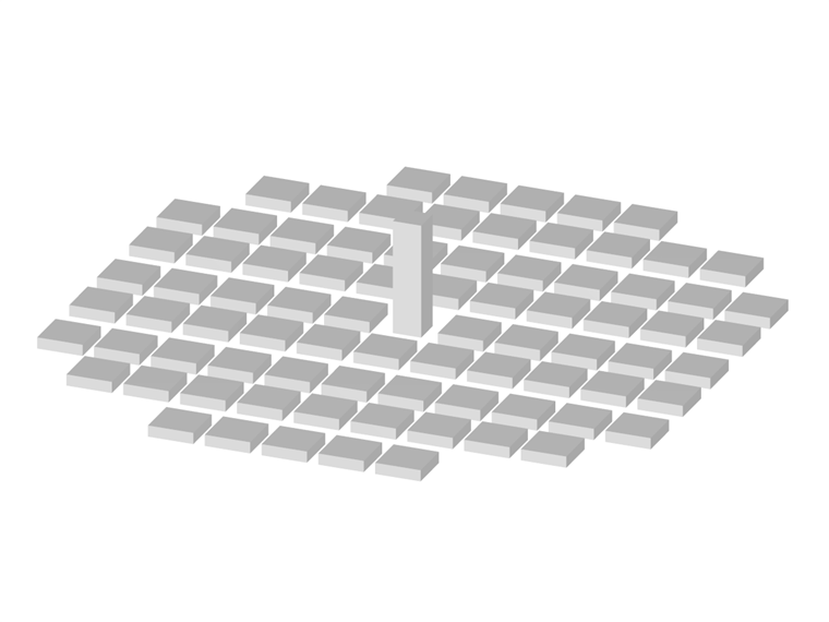
Case D describes a simple cuboid building with a square base and four times the height, surrounded by smaller apartment blocks that are also cuboid.
These apartment blocks also have a rectangular, but larger, floor area, however, with only one-tenth the height of the large building.
The large central building is surrounded by smaller apartment blocks in a regular pattern.
The exact dimensions, flow velocity, and turbulence behavior were taken from the original publication [1].
The distribution of the flow velocity over the height is shown below.

The flow velocity was evaluated in the simulation at a few points of low altitude.
In the AIJ experiment, a corresponding model was set up in a wind tunnel and the wind speed was measured at the mentioned points using split fiber probes.

The standard k–ε was used as a turbulence model, assuming a steady flow.
The model structure with regard to the dimensions of the geometry is shown below. The height of the small buildings is similar to Figure& 0.25, whereas the individual central building is 2.5.

Model Layout - AIJ Case Study: High-Rise Building Among City Blocks

Model Layout 1 - AIJ Case D

Model Layout 2 - AIJ Case D

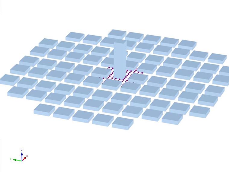
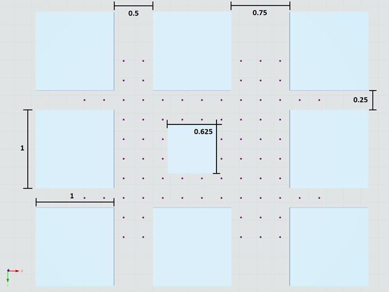
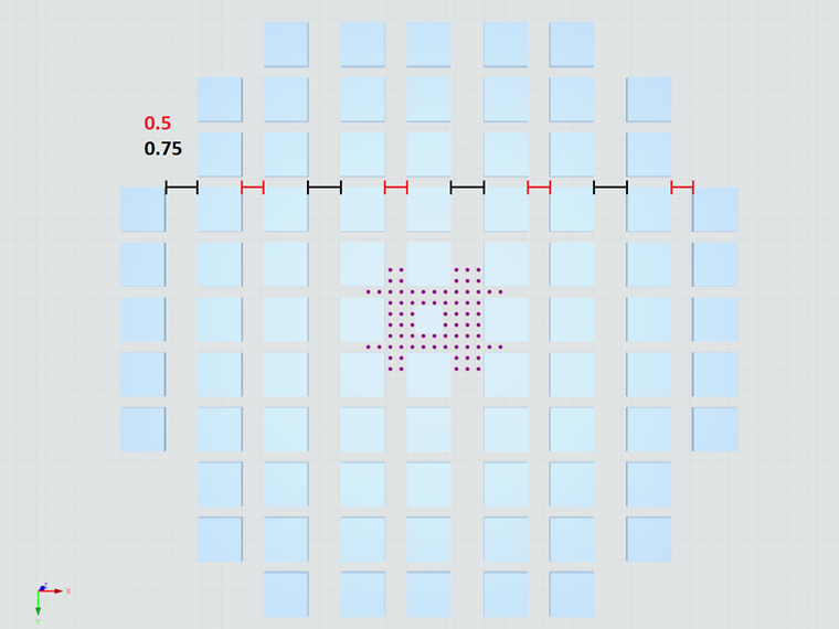
The position of the measuring points is summarized in the following table. The origin is understood in the ground of the city in the center of gravity of the base of the central building. All measuring points are at a height of 0.05.

The experimental results of the AIJ were published on their website [1]. The displayed data of the AIJ simulation were determined using the ENGAUGE Digitizer tool [2] from the plots of the publication [1], since the exact values for this were not published.
However, the accuracy of the extracted points should be sufficiently accurate (in the range +-0.5%) and therefore easily comparable.

In the benchmark experiment, some points were not evaluated, but they were determined in the simulation. In order to avoid having to completely exclude these points from the evaluation, it was assumed that the experiment and the literature simulation yield identical results for these points. For the following comparisons, the results of the literature simulation are even overestimated.

Another important influencing factor is the "Boundary Layers" setting, which significantly increases the mesh density around the lower boundary condition (soil). In general, the meshing close to the ground influences the results in this region more than would be the case with a greater distance to the ground, because the ground boundary condition has a strong influence. Due to the rather complex geometry of the city, the setting mentioned above was activated and the number of extra layers ("NL") set to 10.

RWIND Pro 2.02 was used for this article. The model structure in RWIND was adapted to the structure of the reference CFD as well as possible.

Ergebnisse and Diskussion

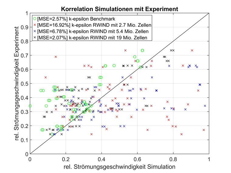
The representation of the three-dimensionally positioned measuring points via simple one-dimensional numbering can be difficult to interpret. Therefore, direct comparisons of the experiment (x-axis) and simulation (y-axis) are shown below for all measuring points. The closer a measuring point is to the diagonal line y=x, the greater the correlation between the simulation and the experiment. Below, there are two of the best-matched RWIND high-element models along with the benchmark from the literature.

Simulation Correlation with Experiment Benchmark and RWIND Simulations with High Number of Elements

It is visible at first glance that the results of the individual measuring points are distributed more homogeneously around the experimental results. While the literature simulation almost always overestimates the flow velocity, RWIND shows sometimes lower, sometimes higher results.

The mean square deviation (MSD) was used as a comparison criterion, but a comparison of the determination coefficients would also show the same behavior, for example. The mean square deviation was preferred to the coefficient of determination because the ratio of experimental and simulated flow velocity does not represent a regression and thus would only be a kind of weighting of individual deviations and not a goodness of fit. The MSD is geometrically easier to interpret with the same expressiveness.

The comparison criterion MSD confirms the presumption of the first observation. Both models with the high mesh resolution, but different turbulence models, meet the experimental benchmark very well. The k-epsilon model is even better than the publication, while the k-omega model is close behind.

However, it should not be forgotten that several points for the literature benchmark were artificially assumed to be faulty.
If these points are calculated for MSD, both RWIND models show a smaller error than the benchmark.

It is advisable to take a closer look at the influence of the mesh density. In the following, meshes of different densities with an otherwise identical model structure and a k-epsilon RAS turbulence model are compared with the literature benchmark. The results are shown below.

Simulation Correlation with Experiment Benchmark and RWIND k-Epsilon Simulations with Different Number of Elements

A mesh convergence study was also carried out for the k-omega turbulence model and the same mesh formations. The results are shown below.

Simulation Correlation with Experiment Benchmark and RWIND k-Omega Simulations with Different Number of Elements

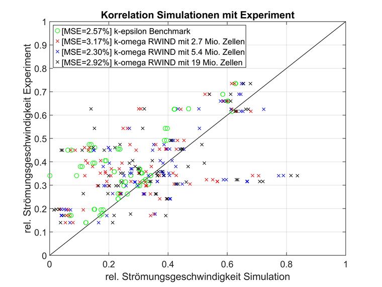
While the k-epsilon RAS turbulence model can achieve slightly better results for very high numbers of elements, the mean square deviation in the k-omega models converges much faster with increasing mesh density. The best example of this is the model pair with 2.7 million cells. Here, the k-epsilon model is quite useless, whereas k-omega can already provide good results.
In fact, the k-omega model with medium resolution comply with the experiment at best and can also outclass the significantly higher-resolution RWIND models. A precise reason for this could not be identified. Therefore, it is possible to assume that the optimization problem with such a high dimensionality is a chance hit.

For a clearer comparison of the reference simulation with the RWIND results, it is advisable to consider the flow velocities as a bottle color image. The considered section around the building was adapted to that of the authors [1]. For copyright reasons, the false color images are not compared side by side at this point. The result is shown below.

Flow Velocity over All Buildings - AIJ Case D

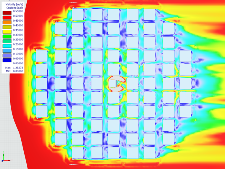
There is also very good correlation with the literature simulation. There are no significant deviations or noticeable areas.

In summary, k-omega is always more accurate for lower-resolution models in this case study, while the results with a high mesh density are still very good.
On the other hand, the pressure residual in the k-omega models converges after significantly more iterations. A comparison is shown below.

Residuals for Two Turbulence Models

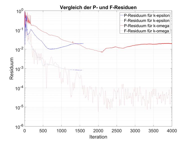
These observations coincide with the expectations of various turbulence models. For the use of k-omega, it is thus recommended to increase the number of maximum iterations considerably. The default value of 300 should be increased manually to at least 1,000.

Summary

The mean square deviations of various combinations of number of elements and turbulence model are summarized below.

A possible improvement approach is often the mesh refinement. In the case of this model, however, the influence of such a mesh refinement is very small. The "Boundary Layers" setting already represents a mesh refinement, so it is possible to sufficiently discretize the relatively small surrounding buildings. The mesh densification analysis was dispensed with after the evaluation of a test model.

Finally, there is very good compliance between RWIND and the experimental benchmark, which can even outclass the literature benchmark. Both turbulence models are suitable for this, whereby the k-omega can provide significantly better results for the low-mesh densities.

[1] https://www.aij.or.jp/jpn/publish/cfdguide/
[2] https://markummitchell.github.io/engauge-digitizer/

• 3D Viewer | Google
• 3D Viewer | Babylon
• Virtual Reality

160x

4x

AIJ Benchmarks Example D – High-Rise Building Surrounded by (Uniform) City Blocks