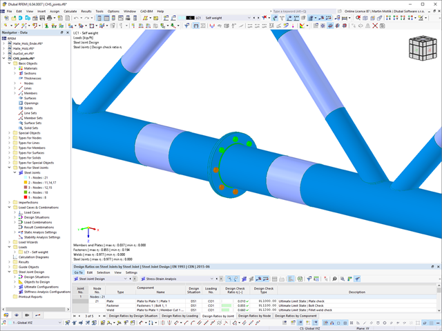
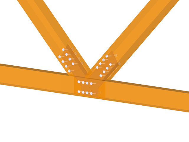
The Steel Joints add-on provides you with the option to connect circular hollow sections using welds.
It is possible to connect the circular sections to each other or to planar structural components. The fillets of standard and thin-walled sections can also be connected with a weld.
Go to Explanatory Video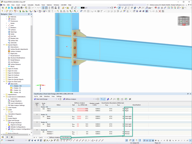
In the Steel Joints add-on, you can classify the joint stiffness.
In addition to the initial stiffness, the table also shows the limit values for hinged and rigid connections for the selected internal forces N, My, and/or Mz. The resulting classification is then displayed in tables as "hinged", "semi-rigid", or "rigid".
Go to Explanatory Video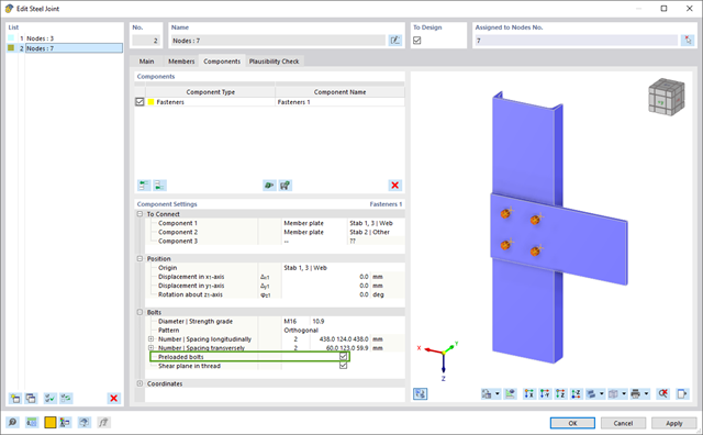
In the "Steel Joints" add-on, you can consider preloaded bolts in all components during the calculation. You can easily activate the preloading using the check box in the bolt parameters, and it has an impact on the stress-strain analysis as well as the stiffness analysis.
Preloaded bolts are special bolts used in steel structures to generate a high clamping force between the connected structural components. This clamping force causes friction between the structural components, which allows for the transfer of forces.
Functionality
Preloaded bolts are tightened with a certain torque, causing them to stretch and generate a tensile force. This tensile force is transferred to the connected components and leads to a high clamping force. The clamping force prevents the connection from loosening and ensures safe force transmission.
Advantages
- High load-bearing capacity: Preloaded bolts can transfer large forces.
- Low deformation: They minimize the deformation of the connection.
- Fatigue strength: They are resistant to fatigue.
- Easy assembly: They are relatively easy to assemble and disassemble.
Analysis and Design
The calculation of preloaded bolts is performed in RFEM using the FE analysis model generated by the "Steel Joints" add-on. It takes into account the clamping force, friction between structural components, shear strength of bolts, and load-bearing capacity of the structural components. The design is carried out according to DIN EN 1993‑1‑8 (Eurocode 3) or the US standard ANSI/AISC 360‑16. You can save the created analysis model, including the results, and use it as an independent RFEM model.
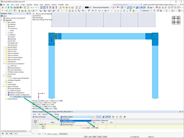
The initial stiffness Sj,ini is a crucial parameter for evaluating whether a connection can be characterized as rigid, semi-rigid, or pinned.
In the "Steel Joints" add-on, you can calculate the initial stiffness Sj,ini according to Eurocode (EN 1993‑1‑8, Section 5.2.2) and AISC (AISC 360-16, Cl. E3.4) with regard to the internal forces N, My, and/or Mz.
The optional automatic transfer of initial stiffnesses allows for a directly transfer as member hinge stiffnesses in RFEM. The entire structure is then recalculated and the resulting internal forces are automatically adopted as loads in the analysis and design of the connection models.
This automated iteration process eliminates the need for manual export and import of data, reducing the amount of work and minimizing potential sources of error.
Explanatory Video: Calculation of Initial Stiffness Sj,ini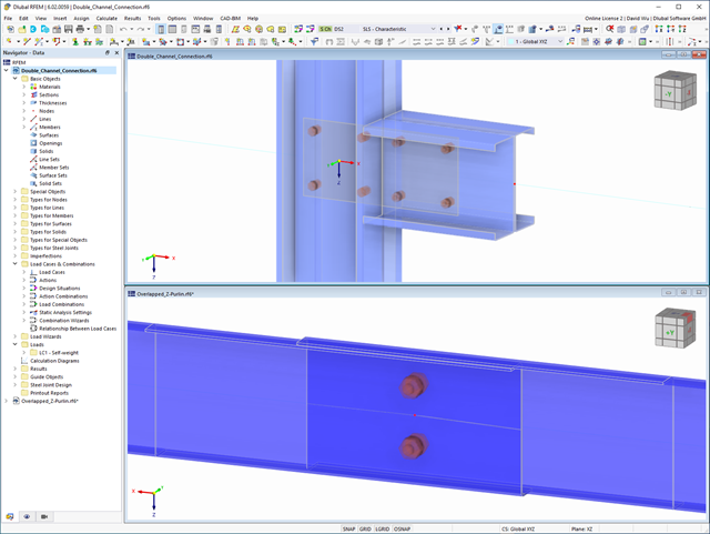
In the Steel Joint add-on, you can design the connections of members with composite cross-sections. Furthermore, you can perform joint design checks for almost all thin-walled cross-sections in the RFEM library.
Go to Explanatory Video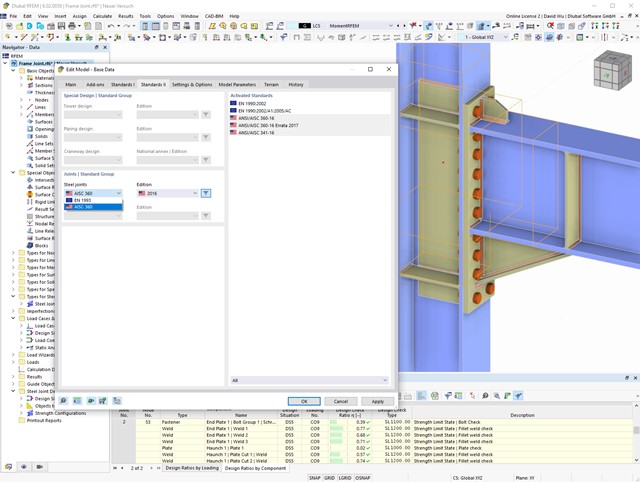
In the Steel Joints add-on, you can design connections according to the American standard ANSI/AISC 360‑16. The following design procedures are integrated:
- Load and Resistance Factor Design (LRFD)
- Allowable Stress Design (ASD)
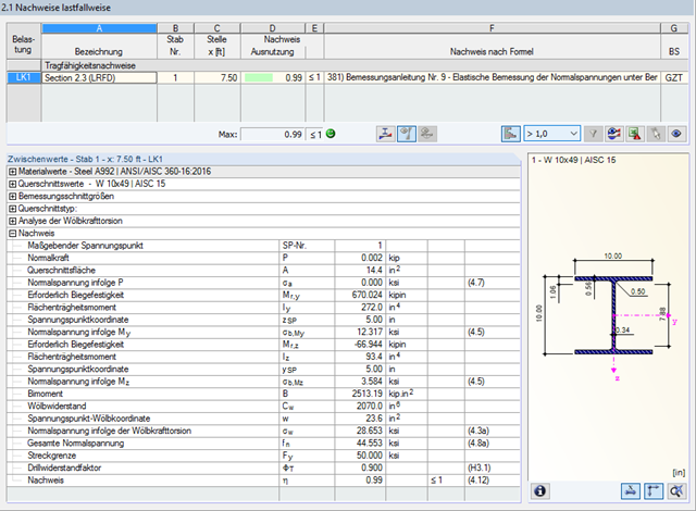
Due to the integrated RF-/STEEL Warping Torsion module extension, it is possible to perform the design according to Design Guide 9 in RF-/STEEL AISC.
The calculation is performed with 7 degrees of freedom according to the warping torsion theory and enables a realistic stability design, including consideration of torsion.
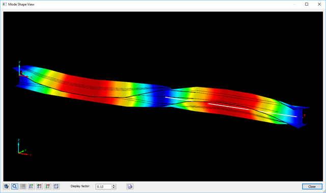
The determination of the critical buckling moment is carried out in RF-/STEEL AISC by using the eigenvalue solver which allows an exact determination of the critical buckling load.
The eigenvalue solver shows a display window of the eigenvalue graphics, which enables checking of the boundary conditions.
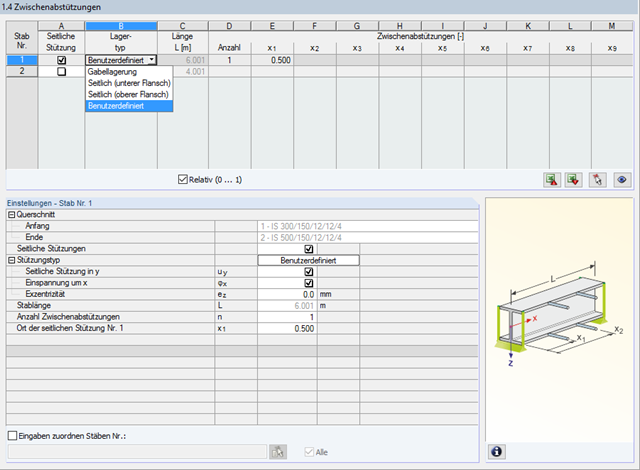
In STEEL AISC, it is possible to consider lateral intermediate supports at any location. For example, it is possible to stabilize only the upper flange.
Furthermore, user-defined lateral intermediate supports can be assigned; for example, single rotational springs and translational springs at any location at the cross-section.
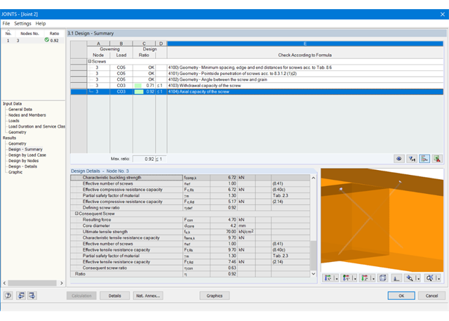
At first, the governing joint designs are arranged in groups and displayed with the basic geometry of the joint in the first result window. In the other result windows, you can see all fundamental design details.
Dimensions, material properties, and welds important for the connection construction are displayed immediately and can be printed directly. Similarly, export to DXF-file is enabled. The connections can be visualized in the RF-/JOINTS Timber - Timber to Timber module as well as in RFEM/RSTAB.
All graphics can be included in the RFEM/RSTAB printout report or printed directly. Due to the scaled output, an optimal visual check is possible as early as in the design phase.
The following design results are displayed:
- Check of minimum spacing
- Load-carrying capacity of each screw
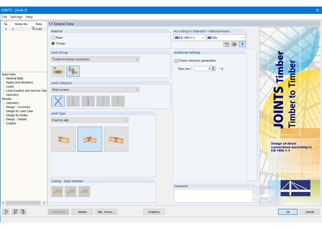
First, select the joint type and the design standard.
The connected members are imported from the RFEM/RSTAB model. The add-on module automatically checks if all geometry conditions are fulfilled.
In addition, the loads are imported automatically from RFEM/RSTAB. In the Geometry window, you can specify the screw parameters (diameter, length, angle, and so on).
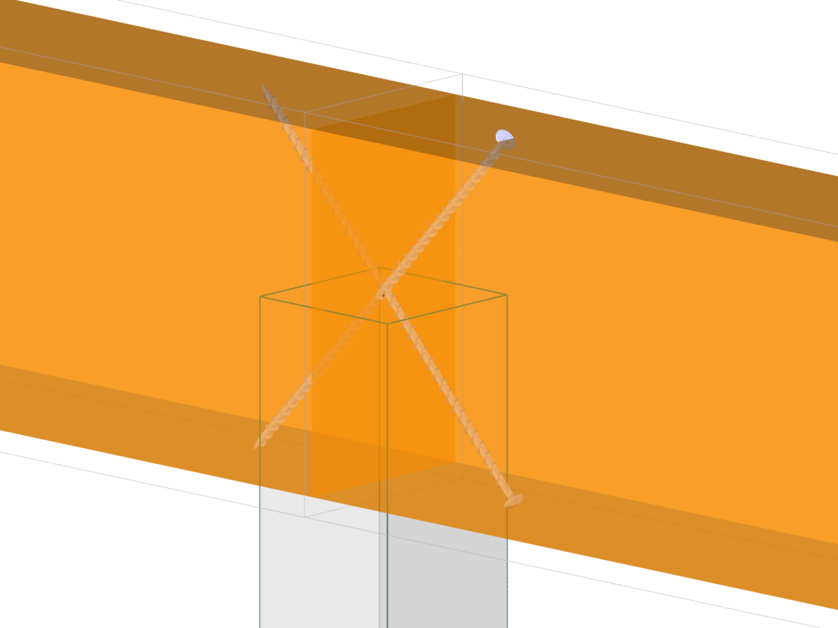.png?mw=640&hash=c1087880acc023575381bb136280b0c348568350)
- Design of hinged connections
- Biaxial inclination of the connected member (for example, a jack rafter joint)
- Connection of any number of members on one node for the type "Main member only"
- Screw diameter 6 mm – 12 mm
- Automatic check of the minimum distance between screws
- Optional free definition of screw distances
- Transfer of eccentricity from RFEM/RSTAB
- Crosswise or parallel screw alignment
- Definition of up to 16 screws in a row
- Graphical visualization of joints in the add-on module and in RFEM/RSTAB
- Performing all required designs
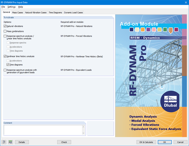
RF-/DYNAM Pro - Nonlinear Time History is integrated in the structure of RF‑/DYNAM Pro - Forced Vibrations and extended by two nonlinear analysis methods (one nonlinear analysis in RSTAB).
Force-time diagrams can be entered as transient, periodic, or as a function of time. Dynamic load cases combine the time diagrams with the static load cases, which provides high flexibility. Furthermore, it is possible to define time steps for the calculation, structural damping, and export options in the dynamic load cases.

- Nonlinear member types, such as tension and compression members or cables
- Member nonlinearities, such as failure, tearing, yielding under tension or compression
- Support nonlinearities, such as failure, friction, diagram, and partial activity
- Release nonlinearities, such as friction, partial activity, diagram, and fixed if positive or negative internal forces
.png?mw=640&hash=8cfd0c4bd093c03de543d147ffbf6f5c9250634a)
- User-defined time diagrams as a function of time, in tabular form, or as harmonic loads
- Combination of the time diagrams with RFEM/RSTAB load cases or combinations (enables definition of nodal, member, and surface loads, as well as free and generated loads varying over time)
- Combination of several independent excitation functions
- Nonlinear time history analysis with the implicit Newmark analysis (RFEM only) or the explicit analysis
- Structural damping using Rayleigh damping coefficients or Lehr's damping
- Direct import of initial deformations from a load case or combination (RFEM only)
- Stiffness modifications as initial conditions; for example, axial force effect, deactivated members (RSTAB only)
- Graphical display of results in a time history diagram
- Export of results in user-defined time steps or as an envelope
- Modeling of the cross-section via elements, sections, arcs, and point elements
- Expansible library of material properties, yield strengths, and limit stresses
- Section properties of open, closed, or non-connected cross-sections
- Ideal section properties of cross-sections consisting of different materials
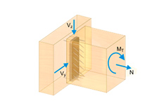
- Determination of weld stresses in fillet welds
- Stress analysis including design of primary and secondary torsion
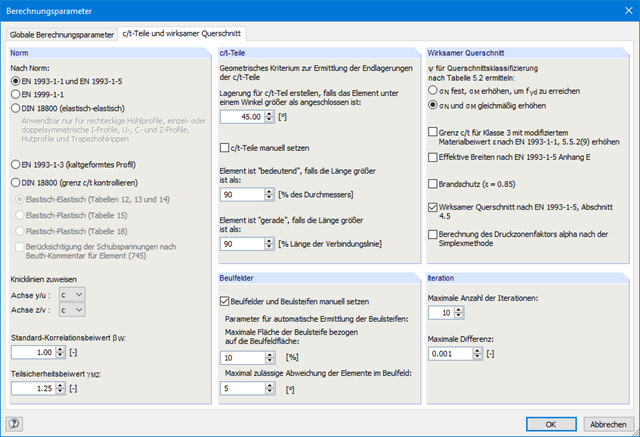
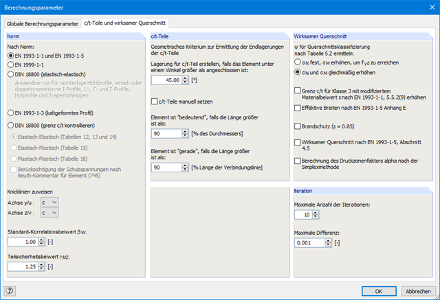
- Check of c/t-ratios
- Effective cross-sections according to
- EN 1993-1-5 (including stiffened buckling panels according to Section 4.5)
-
 EN 1993-1-3
 -
EN 1999-1-1
-
 to DIN 18800-2
- Classification according to
-
EN 1993-1-1
-
EN 1999-1-1
-
- Interface with MS Excel to import and export tables
- Printout report
All results can be evaluated and visualized in an appealing numerical and graphical form. Selection functions facilitate the targeted evaluation.
The printout report corresponds to the high standards of RFEM and rstab/rstab-9/what-is-rstab RSTAB. Modifications are updated automatically.
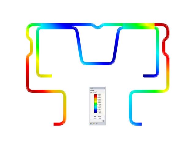
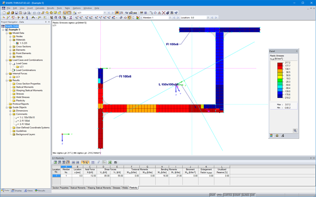
SHAPE-THIN calculates all relevant cross‑section properties, including plastic limit internal forces. Overlapping areas are set close to reality. If cross-sections consist of different materials, SHAPE‑THIN determines the effective cross‑section properties with respect to the reference material.
In addition to the elastic stress analysis, you can perform the plastic design including interaction of internal forces for any cross‑section shape. The plastic interaction design is carried out according to the Simplex Method. You can select the yield hypothesis according to Tresca or von Mises.
SHAPE-THIN performs a cross-section classification according to EN 1993-1-1 and EN 1999-1-1. For steel cross-sections of cross-section class 4, the program determines effective widths for unstiffened or stiffened buckling panels according to EN 1993-1-1 and EN 1993-1-5. For aluminum cross-sections of cross-section class 4, the program calculates effective thicknesses according to EN 1999-1-1.
Optionally, SHAPE‑THIN checks the limit c/t-values in compliance with the design methods el‑el, el‑pl, or pl‑pl according to DIN 18800. The c/t-zones of elements connected in the same direction are recognized automatically.
SHAPE-THIN includes an extensive library of rolled and parameterized cross-sections. They can be composed or supplemented by new elements. It is possible to model a section consisting of different materials.
Graphical tools and functions allow for modeling complex section shapes in the usual way common for CAD programs. The graphical entry provides the option of setting point elements, fillet welds, arcs, parameterized rectangular and circular sections, ellipses, elliptical arcs, parabolas, hyperbolas, spline, and NURBS. Alternatively, it is possible to import a DXF file that is used as the basis for further modeling. You can also use guidelines for modeling.
Furthermore, parameterized input allows you to enter model and load data in a specific way so they depend on certain variables.
Elements can be divided or attached to other objects graphically. SHAPE-THIN automatically divides the elements and provides for an uninterrupted shear flow by introducing dummy elements. In the case of dummy elements, you can define a specific thickness to control the shear transfer.
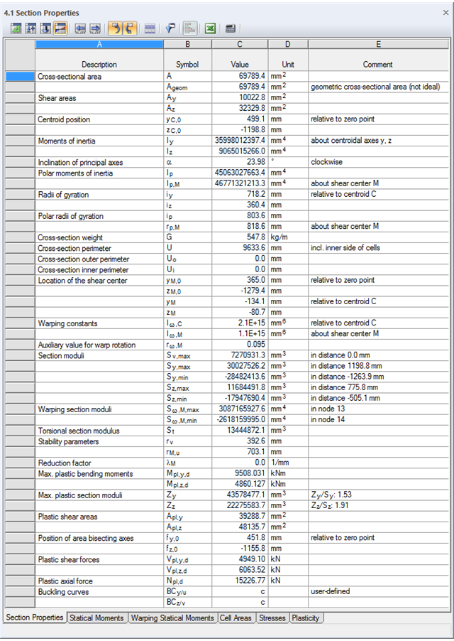
SHAPE-THIN determines the section properties and stresses of any open, closed, built-up, or non-connected cross-sections.
- Section Properties
- Cross-sectional area A
- Shear areas Ay, Az, Au, and Av
- Centroid position yS, zS
- moments of area 2 degrees Iy, Iz, Iyz, Iu, Iv, Ip, Ip,M
- Radii of gyration iy, iz, iyz, iu, iv, ip, ip,M
- Inclination of principal axes α
- Cross-section weight G
- Cross-section perimeter U
- torsional constants of area degrees IT, IT,St.Venant, IT,Bredt, IT,s
- Location of the shear center yM, zM
- Warping constants Iω,S, Iω,M or Iω,D for lateral restraint
- Max/min section moduli Sy, Sz, Su, Sv, Sω,M with locations
- Section ranges ru, rv, rM,u, rM,v
- Reduction factor λM
- Plastic Cross-Section Properties
- Axial force Npl,d
- Shear forces Vpl,y,d, Vpl,z,d, Vpl,u,d, Vpl,v,d
- Bending moments Mpl,y,d, Mpl,z,d, Mpl,u,d, Mpl,v,d
- Section moduli Zy, Zz, Zu, Zv
- Shear areas Apl,y, Apl,z, Apl,u, Apl,v
- Position of area bisecting axes fu, fv,
- Display of the inertia ellipse
- First moments of area Qu, Qv, Qy, Qz with location of maxima and specification of shear flow
- Warping coordinates ωM
- moments of area (warping areas) Sω,M
- Cell areas Am of closed cross-sections
- Normal stresses σx due to axial force, bending moments, and warping bimoment
- Shear stresses τ from shear forces as well as primary and secondary torsional moments
- Equivalent stresses σv with customizable factor for shear stresses
- Stress ratios, related to limit stresses
- Stresses for element edges or center lines
- Weld stresses in fillet welds
- Section properties of non-connected cross-sections (cores of high-rise buildings, composite sections)
- Shear wall shear forces due to bending and torsion
- Plastic capacity design with determination of the enlargement factor αpl
- Check of the c/t-ratios following the design methods el-el, el-pl or pl-pl according to DIN 18800
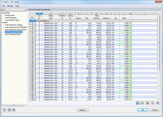
First, the governing design checks of the connection for the respective load case, and load combination, or result combination are displayed. In addition, it is possible to display results separately for sets of members, surfaces, cross-section, members, nodes, and nodal supports.
- You can use a filter to further reduce the displayed results and thus present them in a clearer way.
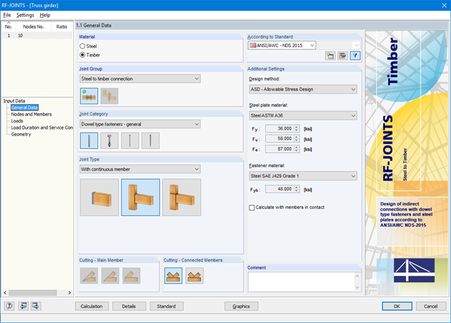
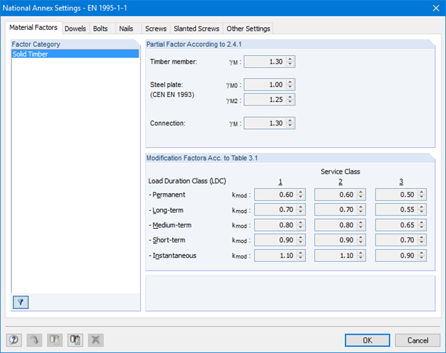
First, it is necessary to select the joint type, design standard, and steel plate and dowel material. For design according to EN 1995-1-1, you can select the SFS intec dowel system WS‑T. In this case, the corresponding material is preset in accordance with the technical approval of the manufacturer.
The connected members are imported from the RFEM/RSTAB model. The add-on module automatically checks if all geometry conditions are fulfilled. Alternatively, you can define the connection manually.
- The loading is also imported from RFEM/RSTAB or, in the case of manual joint definition, loads are entered. The Geometry window includes steel plate dimensions and fastener layouts.
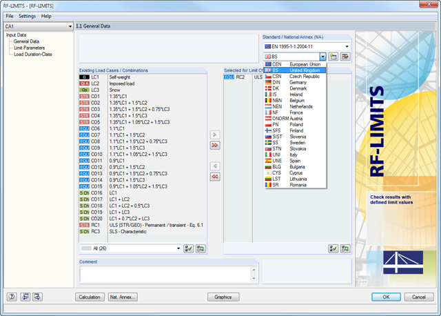
After selecting the loads required for the design and, if necessary, the desired standard for the design, you can define the limit loads in Window 1.2 Limit Parameters. In addition to the manufacturers listed in the limit library, it is possible to add user-defined entries.
After selecting all limit elements for the design, you can optionally define the load duration class (LDC). However, this module window is available only for timber fastener design according to EN 1995-1-1 or DIN 1052.
After the calculation, the RF‑/JOINTS Timber - Steel to Timber add‑on module lists joint stiffnesses of all individual members, among other things. The following design results are displayed:
- Check of minimum spacing
- Load-carrying capacity of single fastener
- Steel plates (bearing resistance and stress according to EC 3 and AISC)
- Stress analysis with reduced timber cross‑section
- Block shear failure
- Total load carrying-capacity (including stiffness determination, transversal tension design according to EC 5, and others)
- Fire resistance design according to EN 1995‑1‑2
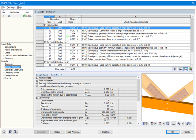
At first, the governing joint designs are arranged in groups and displayed with the basic geometry of the joint in the first result window. In the other result windows, you can see all fundamental design details.
Dimensions, material properties, and welds important for the connection construction are displayed immediately and can be printed directly. Similarly, export to DXF-file is enabled. It is possible to visualize the connections in RF‑/JOINTS Timber - Steel to Timber or in the RFEM/RSTAB model.
All graphics can be included in the RFEM/RSTAB printout report or printed directly. Due to the scaled output, an optimal visual check is possible as early as in the design phase.
- Design of hinged, bending resistant, and semi-rigid connections
- Definition of up to 5 steel plates slotted in timber beams
- Up to 8 members connected to one node
- Thickness of steel plate 5 mm – 40 mm
- All sizes of fasteners
- Automatic check of the minimum distance between fasteners
- Optional free definition of fastener distances
- Definition of asymmetrical fastener arrangements (for example, any polygonal chains)
- Graphical visualization of joints in the add-on module and in RFEM/RSTAB
- All required steel and timber designs, including reduction of cross‑section values
- Design of transversal tension reinforcement (for EN 1995‑1‑1 only)
- Export of the member eccentricities to RFEM/RSTAB to be considered in the determination of internal forces
- Dowel length optionally shorter than cross-section width (for wooden plugs)
- DXF Export of Connection Geometry
- Fire resistance design according to EN 1995‑1‑2
- Design of member ends, members, nodal supports, nodes, and surfaces
- Consideration of specified design areas
- Check of cross-section dimensions
- Design according to EN 1995-1-1 (European Timber Standard) with the respective National Annexes + DIN 1052 + DSTV DIN EN 1993-1-8 + ANSI / AWC - NDS 2015 (US Standard)
- Design of various materials, such as steel, concrete, and others
- No necessary linking to specific standards
- Extensible library including timber fasteners (SIHGA, Sherpa, WÜRTH, Simpson StrongTie, KNAPP, PITZL) and steel fasteners (standardized connections in steel building design according to EC 3, M-connect, PFEIFER, TG-Technik)
- Ultimate load capacities of timber beams by the companies STEICO and Metsä Wood available in the library
- Connection to MS Excel
- Optimization of connecting elements (the most utilized element is calculated)