44 Results
View Results:
Sort by:

As you've already learned, the results of a Modal Analysis load case are displayed in the program after a successful calculation. You can thus immediately see the first mode shape graphically or as an animation. You can also easily adjust the representation of the mode shape standardization. Do that directly in the Results navigator, where you have one of four options for the visualization of the mode shapes available for the selection:
- Scaling the value of the mode shape vector uj to 1 (considers the translation components only)
- Selecting the maximum translational component of the eigenvector and setting it to 1
- Considering the entire eigenvector (including the rotation components), selecting the maximum, and setting it to 1
- Setting the modal mass mi for each mode shape to 1 kg
You can find a detailed explanation of the mode shape standardization in the OnlineManual here.
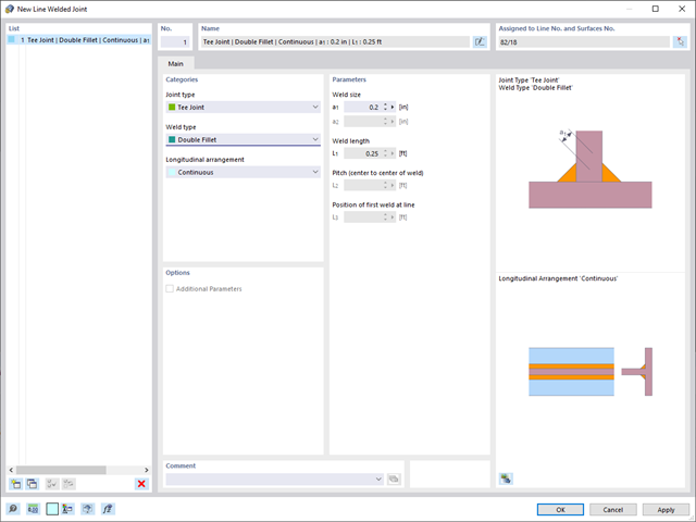
In RFEM 6, it is possible to define line welds between surfaces and to calculate the weld stresses using the Stress-Strain Analysis add-on.
The following joint types are available:
- Butt Joint
- Corner joint
- Lap Joint
- T-joint
Depending on the selected joint type, you can select the following weld types:
- Single Square
- Double Square
- Double Bevel
- Single V
- Double V
- Single U
- Double U
- Single J
- Double J

RFEM allows you to use a special line hinge to model the special properties of the connection between the reinforced concrete slab and masonry wall. This limits the transferable forces of the connection depending on the specified geometry. You guess right: This means that the material cannot be overloaded.
The program develops interaction diagrams that are applied automatically. They represent the various geometric situations and you can use them to determine the correct stiffness.

Is the calculation finished? The results of the modal analysis are then available both graphically and in tables. Display the result tables for the load case or the load cases of the modal analysis. Thus, you can see the eigenvalues, angular frequencies, natural frequencies, and natural periods of the structure at first glance. The effective modal masses, modal mass factors, and participation factors are also clearly displayed.

Compared to the RF‑/STEEL add-on module (RFEM 5 / RSTAB 8), the following new features have been added to the Stress-Strain Analysis add-on for RFEM 6 / RSTAB 9:
- Treatment of members, surfaces, solids, welds (line welded joints between two and three surfaces with subsequent stress design)
- Output of stresses, stress ratios, stress ranges, and strains
- Limit stress depending on the assigned material or a user-defined input
- Individual specification of the results to be calculated through freely assignable setting types
- Non-modal result details with prepared formula display and additional result display on the cross-section level of members
- Output of the design check formulas used

After you have completed the design, the program takes care of clearly arranged results. Thus, the program shows you the resulting maximum stresses and stress ratios sorted by section, member/surface, solid, member set, x-location, and so on. In addition to the tabular result values, the add-on shows you the corresponding cross-section graphic with stress points, stress diagram, and values as well. You can relate the design ratio to any kind of stress type. The current location is highlighted in the RFEM/RSTAB model.
In addition to the tabular evaluation, the program offers you even more. You can also graphically check the stresses and design ratios on the RFEM/RSTAB model. It is possible for you to adjust the colors and values individually.
The display of result diagrams of a member or set of members enables you a targeted evaluation. For each design location, you can open the respective dialog box to check the design-relevant section properties and stress components of any stress point. Finally, you have the option of printing the corresponding graphic, including all design details.

Is your goal to determine the number of mode shapes? The program offers you two methods for this. On the one hand, you can manually define the number of the smallest mode shapes to be calculated. In this case, the number of available mode shapes depends on the degrees of freedom (that is, the number of free mass points multiplied by the number of directions in which the masses act). However, it is limited to 9999. On the other hand, you can set the maximum natural frequency the way that the program determined the mode shapes automatically until reaching the natural frequency set.
.png?mw=640&hash=25998fe3470f8e1c154828f202ad6a728b30f00a)
Did you know that To calculate masonry structures, a nonlinear material model has been implemented in RFEM. It is based on the approach of Lourenco, a composite yield surface according to Rankine and Hill. This model allows you to describe and model the structural behavior of masonry and the different failure mechanisms.
The limit parameters were selected in such a way that the design curves used correspond to a normative design curve.

The Concrete Design add-on allows you to perform the seismic design of reinforced concrete members according to EC 8. This includes, among other things, the following functionalities:
- Seismic design configurations
- Differentiation of the ductility classes DCL, DCM, DCH
- Option to transfer the behavior factor from a dynamic analysis
- Check of the limit value for the behavior factor
- Capacity design checks of "Strong column - weak beam"
- Detailing and particular rules for curvature ductility factor
- Detailing and particular rules for local ductility

You can select several methods that are available for the eigenvalue analysis:
- Direct Methods
- The direct methods (Lanczos [RFEM], roots of characteristic polynomial [RFEM], subspace iteration method [RFEM/RSTAB], and shifted inverse iteration [RSTAB]) are suitable for small to medium-sized models. You should only use these fast solver methods if your computer has a larger amount of memory (RAM).
- ICG Iteration Method (Incomplete Conjugate Gradient [RFEM])
- In contrast, this method only requires a small amount of memory. Eigenvalues are determined one after the other. It can be used to calculate large structural systems with few eigenvalues.
Use the Structure Stability add-on to perform a nonlinear stability analysis using the incremental method. This analysis delivers close-to-reality results also for nonlinear structures. The critical load factor is determined by gradually increasing the loads of the underlying load case until the instability is reached. The load increment takes into account nonlinearities such as failing members, supports and foundations, and material nonlinearities. After increasing the load, you can optionally perform a linear stability analysis on the last stable state in order to determine the stability mode.

Compared to the RF‑/STABILITY (RFEM 5) and RSBUCK (RSTAB 8) add-on modules, the following new features have been added to the Structure Stability add-on for RFEM 6 / RSTAB 9:
- Activation as a property of a load case or a load combination
- Automated activation of the stability calculation via combination wizards for several load situations in one step
- Incremental load increase with user-defined termination criteria
- Modification of the mode shape normalization without recalculation
- Result tables with filter option
.png?mw=640&hash=8b43c740f4a91092df759928a6ee21f06f78f8cc)
The calculation of masonry is carried out in compliance with the nonlinear-plastic material law. If the load at any point is higher than the possible load to be resisted, redistribution takes place within the system. This have the simple purpose of restoring the equilibrium of forces. With the successful completion of the calculation, the stability analysis is provided.

Have you already discovered the tabular and graphical output of masses in mesh points? That's right, this is also part of the modal analysis results in RFEM 6. This way, you can check the imported masses that depend on various settings of the modal analysis. They can be displayed in the Masses in Mesh Points tab of the Results table. The table provides you with an overview of the following results: Mass - Translational Direction (mX, mY, mZ), Mass - Rotational Direction (mφX, mφY, mφZ), and the Sum of Masses. Would it be best for you to have a graphical evaluation as quickly as possible? Then you can also graphically display the masses in mesh points.
- Determination of principal and basic stresses, membrane and shear stresses, as well as equivalent stresses and equivalent membrane stresses
- Stress analysis for structural surfaces including simple or complex shapes
- Equivalent stresses calculated according to different approaches:
- Shape modification hypothesis (von Mises)
- Shear stress hypothesis (Tresca)
- Normal stress hypothesis (Rankine)
- Principal strain hypothesis (Bach)
- Optional optimization of surface thicknesses and data transfer to RFEM
- Output of strains
- Detailed results of individual stress components and ratios in tables and graphics
- Filter function for solids, surfaces, lines, and nodes in tables
- Transversal shear stresses according to Mindlin, Kirchhoff, or user-defined specifications
- Stress evaluation for welds at connection lines between surfaces (see the Product Feature)

As the first results, the program presents you with the critical load factors. You can then perform an evaluation of stability risks. For member models, the resulting effective lengths and critical loads of the members are displayed to you in tables.
Use the next result window to check the normalized eigenvalues sorted by node, member, and surface. The eigenvalue graphic allows you to evaluate the buckling behavior. This makes it easier for you to take countermeasures.

Was your design successful? Then just sit back and relax. You benefit from the numerous functions in RFEM also here. The program gives you the maximum stresses of the masonry surfaces, whereby you can display the results in detail at each FE mesh point.
Moreover, you can insert sections in order to carry out a detailed evaluation of the individual areas. Use the display of the yield areas to estimate the cracks in the masonry.
If there is a load case or load combination in the program, the stability calculation is activated. You can define another load case in order to consider initial prestress, for example.
For this, you need to specify whether to perform a linear or nonlinear analysis. Depending on the case of application, you can select a direct calculation method, such as the Lanczos method or the ICG iteration method. Members not integrated in surfaces are usually displayed as member elements with two FE nodes. With such elements, the program cannot determine the local buckling of single members. That's why you have the option to divide members automatically.

Did you know? You can easily define structural modifications in load cases of the Modal Analysis type. This allows you, for example, to individually adjust the stiffnesses of materials, cross-sections, members, surfaces, hinges, and supports. You can also modify stiffnesses for some design add-ons. Once you select the objects, their stiffness properties are adapted to the object type. In this way, you can define them in separate tabs.
Do you want to analyze the failure of an object (for example, a column) in the modal analysis? This is also possible without any problems. Simply switch to the Structure Modification window and deactivate the relevant objects.

- Stress determination using an elastic-plastic material model
- Design of masonry disc structures for compression and shear on the building model or single model
- Automatic determination of stiffness of a wall-slab hinge
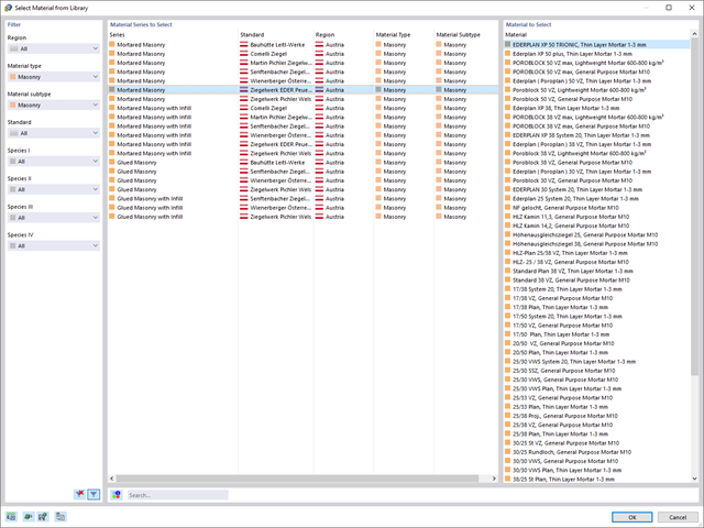
- An extensive material database for almost all stone-mortar combinations available on the Austrian market (the product range is continuously being expanded, for other countries as well)
- Automatic determination of material values according to Eurocode 6 (ÖN EN 1996‑X)
- Option to create pushover analysis
You enter and model the structure directly in RFEM. You can combine the masonry material model with all common RFEM add-ons. This enables you to design the entire building models in connection with masonry.
The program automatically determines for you all parameters required for the calculation by using the material data that you have entered. Then, it finally generates the stress-strain curves for each FE element.