
If there is a load case or load combination in the program, the stability calculation is activated. You can define another load case in order to consider initial prestress, for example.
For this, you need to specify whether to perform a linear or nonlinear analysis. Depending on the case of application, you can select a direct calculation method, such as the Lanczos method or the ICG iteration method. Members not integrated in surfaces are usually displayed as member elements with two FE nodes. With such elements, the program cannot determine the local buckling of single members. That's why you have the option to divide members automatically.

You can select several methods that are available for the eigenvalue analysis:
- Direct Methods
- The direct methods (Lanczos [RFEM], roots of characteristic polynomial [RFEM], subspace iteration method [RFEM/RSTAB], and shifted inverse iteration [RSTAB]) are suitable for small to medium-sized models. You should only use these fast solver methods if your computer has a larger amount of memory (RAM).
- ICG Iteration Method (Incomplete Conjugate Gradient [RFEM])
- In contrast, this method only requires a small amount of memory. Eigenvalues are determined one after the other. It can be used to calculate large structural systems with few eigenvalues.
Use the Structure Stability add-on to perform a nonlinear stability analysis using the incremental method. This analysis delivers close-to-reality results also for nonlinear structures. The critical load factor is determined by gradually increasing the loads of the underlying load case until the instability is reached. The load increment takes into account nonlinearities such as failing members, supports and foundations, and material nonlinearities. After increasing the load, you can optionally perform a linear stability analysis on the last stable state in order to determine the stability mode.

As the first results, the program presents you with the critical load factors. You can then perform an evaluation of stability risks. For member models, the resulting effective lengths and critical loads of the members are displayed to you in tables.
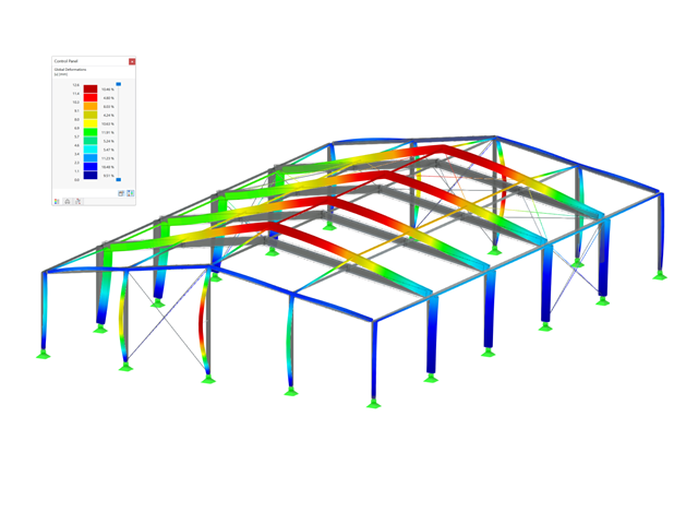
Use the next result window to check the normalized eigenvalues sorted by node, member, and surface. The eigenvalue graphic allows you to evaluate the buckling behavior. This makes it easier for you to take countermeasures.

- Calculation of models consisting of member, shell, and solid elements
- Nonlinear stability analysis
- Optional consideration of axial forces from initial prestress
- Four equation solvers for an efficient calculation of various structural models
- Optional consideration of stiffness modifications in RFEM/RSTAB
- Determination of a stability mode greater than the user-defined load increment factor (Shift method)
- Optional determination of the mode shapes of unstable models (to identify the cause of instability)
- Visualization of the stability mode
- Basis for determining imperfection

- General stress analysis
- Automatic import of internal forces from RFEM/RSTAB
- Graphical and numerical output of stresses, strains, clearance, and design ratios fully integrated in RFEM/RSTAB
- User-defined specification of the limit stress
- Summary of similar structural components for the design
- Wide range of customization options for graphical output
- Clearly arranged result tables for a quick overview after the design
- Simple traceability of the results due to the complete documentation of the calculation method including all formulas
- High productivity due to the minimal amount of input data required
- Flexibility due to detailed setting options for basis and extent of calculations
- Gray zone display for unimportant value ranges (see Product Feature)

- Cross-section optimization
- Transfer of optimized sections to RFEM/RSTAB
- Design of any thin-walled section from RSECTION
- Representation of a stress diagram on a section
- Determination of normal, shear, and equivalent stresses
- Output of stress components for the individual member internal force types
- Detailed representation of stresses in all stress points
- Determination of the largest Δσ for each stress point (for example, for fatigue design)
- Colored display of stresses and design ratios for a quick overview of the critical or oversized zones
- Output of parts lists

- Determination of principal and basic stresses, membrane and shear stresses, as well as equivalent stresses and equivalent membrane stresses
- Stress analysis for structural surfaces including simple or complex shapes
- Equivalent stresses calculated according to different approaches:
- Shape modification hypothesis (von Mises)
- Shear stress hypothesis (Tresca)
- Normal stress hypothesis (Rankine)
- Principal strain hypothesis (Bach)
- Optional optimization of surface thicknesses and data transfer to RFEM
- Output of strains
- Detailed results of individual stress components and ratios in tables and graphics
- Filter function for solids, surfaces, lines, and nodes in tables
- Transversal shear stresses according to Mindlin, Kirchhoff, or user-defined specifications
- Stress evaluation for welds at connection lines between surfaces (see the Product Feature)

After you have completed the design, the program takes care of clearly arranged results. Thus, the program shows you the resulting maximum stresses and stress ratios sorted by section, member/surface, solid, member set, x-location, and so on. In addition to the tabular result values, the add-on shows you the corresponding cross-section graphic with stress points, stress diagram, and values as well. You can relate the design ratio to any kind of stress type. The current location is highlighted in the RFEM/RSTAB model.
In addition to the tabular evaluation, the program offers you even more. You can also graphically check the stresses and design ratios on the RFEM/RSTAB model. It is possible for you to adjust the colors and values individually.
The display of result diagrams of a member or set of members enables you a targeted evaluation. For each design location, you can open the respective dialog box to check the design-relevant section properties and stress components of any stress point. Finally, you have the option of printing the corresponding graphic, including all design details.
- A wide range of available sections, such as rolled I-sections; channel sections; T-sections; angles; rectangular and circular hollow sections; round bars; symmetrical and asymmetrical, parametric I-, T-, and angle sections; built-up cross-sections (suitability for design depends on the selected standard)
- Design of general RSECTION cross-sections (depending on the design formats available in the respective standard); for example, equivalent stress design
- Design of tapered members (design method depending on the standard)
- Adjustment of the essential design factors and standard parameters is possible
- Flexibility due to detailed setting options for basis and extent of calculations
- Fast and clear results output for an immediate overview of the result distribution after the design
- Detailed output of the design results and essential formulas (comprehensible and verifiable result path)
- Numerical results clearly arranged in tables and graphical display of the results in the model
- Integration of the output into the RFEM/RSTAB printout report
- Design of tension, compression, bending, shear, torsion, and combined internal forces
- Tension design with consideration of a reduced section area (for example, hole weakening)
- Automatic classification of cross-sections to check local buckling
- Internal forces from the calculation with Torsional Warping (7 DOF) are taken into account by means of the equivalent stress check (currently not yet for the design standard ADM 2020).
- Design of cross-sections of Class 4 with effective cross-section properties according to EN 1993‑1‑5 (licenses for RSECTION and Effective Sections are required for the RSECTION cross-sections)
- Shear buckling check with consideration of transverse stiffeners

- Stability analyses for flexural buckling, torsional buckling, and flexural-torsional buckling under compression
- Lateral-torsional buckling analysis of the structural components subjected to moment loading
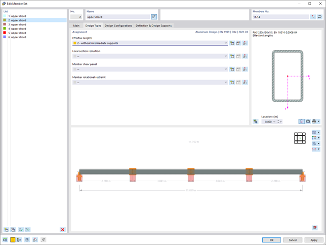
- Import of the effective lengths from the calculation using the Structure Stability add-on
- Graphical input and check of the defined nodal supports and effective lengths for stability analysis
- Depending on the standard, a choice between user-defined input of Mcr, analytical method from the standard, and use of internal eigenvalue solver
- Consideration of a shear panel and a rotational restraint when using the eigenvalue solver
- Graphical display of a mode shape if the eigenvalue solver was used
- Stability analysis of structural components with the combined compression and bending stress, depending on the design standard
- Comprehensible calculation of all necessary coefficients, such as interaction factors
- Alternative consideration of all effects for the stability analysis when determining internal forces in RFEM/RSTAB (second-order analysis, imperfections, stiffness reduction, possibly in combination with the Torsional Warping (7 DOF) add-on)

The parameters of the National Annexes (NA) to Eurocode 3 of the following countries are integrated:
-
 DIN EN 1993-1-1/NA:2016-04 (Germany)
 -
 ÖNORM EN 1993-1-1/NA:2015-12 (Austria)
 -
 SN EN 1993-1-1/NA:2016-07 (Switzerland)
 -
 BDS EN 1993-1-1/NA:2015-10 (Bulgaria)
 -
 BS EN 1993-1-1/NA:2016-07 (United Kingdom)
 -
 CEN EN 1993-1-1/2015-06 (European Union)
 -
 CYS EN 1993-1-1/NA:2015-07 (Cyprus)
 -
 CSN EN 1993-1-1/NA:2016-06 (Czech Republic)
 -
 DS EN 1993-1-1/NA:2015-07 (Denmark)
 -
 ELOT EN 1993-1-1/NA:2017-01 (Greece)
 -
 EVS EN 1993-1-1/NA:2015-08 (Estonia)
 -
 HRN EN 1993-1-1/NA:2016-03 (Croatia)
 -
 I S. EN 1993-1-1/NA:2016-03 (Ireland)
 -
 ILNAS EN 1993-1-1/NA:2015-06 (Luxembourg)
 -
 IST EN 1993-1-1/NA:2015-11 (Iceland)
 -
 LST EN 1993-1-1/NA:2017-01 (Lithuania)
 -
 LVS EN 1993-1-1/NA:2015-10 (Latvia)
 -
 MS EN 1993-1-1/NA:2010-01 (Malaysia)
 -
 MSZ EN 1993-1-1/NA:2015-11 (Hungary)
 -
 NBN EN 1993-1-1/NA:2015-07 (Belgium)
 -
 NEN EN 1993-1-1/NA:2016-12 (Netherlands)
 -
 NF EN 1993-1-1/NA:2016-02 (France)
 -
 NP EN 1993-1-1/NA:2009-03 (Portugal)
 -
 NS EN 1993-1-1/NA:2015-09 (Norway)
 -
 PN EN 1993-1-1/NA:2015-08 (Poland)
 -
 SFS EN 1993-1-1/NA:2015-08 (Finland)
 -
 SIST EN 1993-1-1/NA:2016-09 (Slovenia)
 -
 SR EN 1993-1-1/NA:2016-04 (Romania)
 -
 SS EN 1993-1-1/NA:2019-05 (Singapore)
 -
 SS EN 1993-1-1/NA:2015-06 (Sweden)
 -
 STN EN 1993-1-1/NA:2015-10 (Slovakia)
 -
 TKP EN 1993-1-1/NA:2015-04 (Belarus)
 -
 UNE EN 1993-1-1/NA:2016-02 (Spain)
 -
 UNI EN 1993-1-1/NA:2015-08 (Italy)

- Realistic representation of interaction between a building and soil
- Realistic representation of the influences of the foundation components on each other
- Extensible library of soil properties
- Consideration of several soil samples (probes) at different locations, even outside the building
- Determination of settlements and stress diagrams as well as their graphical and tabular display

Entering soil layers for soil samples is performed in a clearly arranged dialog box. A corresponding graphical representation supports clarity and makes checking the input user-friendly.
An extensible database facilitates the selection of soil material properties. The Mohr-Coulomb model as well as a nonlinear model with stress and strain dependent stiffness are available for a realistic modeling of the soil material behavior.
You can define any number of soil samples and layers. The soil is generated from all entered samples using 3D solids. Assignment to the structure is carried out using coordinates.
The soil body is calculated according to the nonlinear iterative method. The calculated stresses and settlements are displayed graphically and in tables.

- Automatic consideration of masses from self-weight
- Direct import of masses from load cases or load combinations
- Optional definition of additional masses (nodal, linear, or surface masses, as well as inertia masses) directly in the load cases
- Optional neglect of masses (for example, mass of foundations)
- Combination of masses in different load cases and load combinations
- Preset combination coefficients for various standards (EC 8, SIA 261, ASCE 7,...)
- Optional import of initial states (for example, to consider prestress and imperfection)
- Structure Modification
- Consideration of failed supports or members/surfaces/solids
- Definition of several modal analyses (for example, to analyze different masses or stiffness modifications)
- Selection of mass matrix type (diagonal matrix, consistent matrix, unit matrix), including user-defined specification of translational and rotational degrees of freedom
- Methods for determining the number of mode shapes (user-defined, automatic - to reach effective modal mass factors, automatic - to reach the maximum natural frequency - only available in RSTAB)
- Determination of mode shapes and masses in nodes or FE mesh points
- Results of eigenvalue, angular frequency, natural frequency, and period
- Output of modal masses, effective modal masses, modal mass factors, and participation factors
- Masses in mesh points displayed in tables and graphics
- Visualization and animation of mode shapes
- Various scaling options for mode shapes
- Documentation of numerical and graphical results in printout report

In the modal analysis settings, you have to enter all data that are necessary for the determination of the natural frequencies. These are, for example, mass shapes and eigenvalue solvers.
The Modal Analysis add-on determines the lowest eigenvalues of the structure. Either you adjust the number of eigenvalues or let them determined automatically. Thus, you should reach either effective modal mass factors or maximum natural frequencies. Masses are imported directly from load cases and load combinations. In this case, you have the option to consider the total mass, load components in the global Z-direction, or only the load component in the direction of gravity.
You can manually define additional masses at nodes, lines, members, or surfaces. Furthermore, you can influence the stiffness matrix by importing axial forces or stiffness modifications of a load case or load combination.

In RFEM, you can use these three powerful eigenvalue solvers:
- Root of Characteristic Polynomial
- Method by Lanczos
- Subspace Iteration
RSTAB, on the other hand, provides you with these two eigenvalue solvers:
- Subspace Iteration
- Shifted inverse power method
The selection of the eigenvalue solver depends primarily on your model size.

As soon as the program has completed the calculation, the eigenvalues, natural frequencies and periods are listed. These result windows are integrated in the main program RFEM/RSTAB. You can find all mode shapes of the structure in tables and also have an option to display them graphically and to animate them.
All result tables and graphics are part of the RFEM/RSTAB printout report. In this way, you can ensure clearly arranged documentation. You can also export the tables to MS Excel.

The Dlubal structural analysis software does a lot of work for you. The input parameters, which are relevant for the selected standards, are suggested by the program in accordance with the rules. Furthermore, you can enter response spectra manually.
Load cases of the type Response Spectrum Analysis define the direction in which response spectra act and which eigenvalues of the structure are relevant for the analysis. In the spectral analysis settings, you can define details for the combination rules, damping (if applicable), and zero-period acceleration (ZPA).

Did you know that Equivalent static loads are generated separately for each relevant eigenvalue and excitation direction. These loads are saved in a load case of the Response Spectrum Analysis type and RFEM/RSTAB performs a linear static analysis.