
As you've already learned, the results of a Modal Analysis load case are displayed in the program after a successful calculation. You can thus immediately see the first mode shape graphically or as an animation. You can also easily adjust the representation of the mode shape standardization. Do that directly in the Results navigator, where you have one of four options for the visualization of the mode shapes available for the selection:
- Scaling the value of the mode shape vector uj to 1 (considers the translation components only)
- Selecting the maximum translational component of the eigenvector and setting it to 1
- Considering the entire eigenvector (including the rotation components), selecting the maximum, and setting it to 1
- Setting the modal mass mi for each mode shape to 1 kg
You can find a detailed explanation of the mode shape standardization in the OnlineManual here.

Did you know? In contrast to other material models, the stress-strain diagram for this material model is not antimetric to the origin. You can use this material model to simulate the behavior of steel fiber-reinforced concrete, for example. Find detailed information about modeling steel fiber-reinforced concrete in the technical article about Determining the material properties of steel-fiber-reinforced concrete.
In this material model, the isotropic stiffness is reduced with a scalar damage parameter. This damage parameter is determined from the stress curve defined in the Diagram. The direction of the principal stresses is not taken into account. Rather, the damage occurs in the direction of the equivalent strain, which also covers the third direction perpendicular to the plane. The tension and compression area of the stress tensor is treated separately. In this case, different damage parameters apply.
The "Reference element size" controls how the strain in the crack area is scaled to the length of the element. With the default value zero, no scaling is performed. Thus, the material behavior of the steel fiber concrete is modeled realistically.
Find more information about the theoretical background of the "Isotropic Damage" material model in the technical article describing the Nonlinear Material Model Damage.

Compared to the RF‑/DYNAM Pro - Natural Vibrations add-on module (RFEM 5 / RSTAB 8), the following new features have been added to the Modal Analysis add-on for RFEM 6 / RSTAB 9:
- Preset combination coefficients for various standards (EC 8, ASCE, and so on)
- Optional neglect of masses (for example, mass of foundations)
- Methods for determining the number of mode shapes (user-defined, automatic - to reach effective modal mass factors, automatic - to reach the maximum natural frequency)
- Output of modal masses, effective modal masses, modal mass factors, and participation factors
- Masses in mesh points displayed in tables and graphics
- Various scaling options for mode shapes in the Result navigator

- Automatic consideration of masses from self-weight
- Direct import of masses from load cases or load combinations
- Optional definition of additional masses (nodal, linear, or surface masses, as well as inertia masses) directly in the load cases
- Optional neglect of masses (for example, mass of foundations)
- Combination of masses in different load cases and load combinations
- Preset combination coefficients for various standards (EC 8, SIA 261, ASCE 7,...)
- Optional import of initial states (for example, to consider prestress and imperfection)
- Structure Modification
- Consideration of failed supports or members/surfaces/solids
- Definition of several modal analyses (for example, to analyze different masses or stiffness modifications)
- Selection of mass matrix type (diagonal matrix, consistent matrix, unit matrix), including user-defined specification of translational and rotational degrees of freedom
- Methods for determining the number of mode shapes (user-defined, automatic - to reach effective modal mass factors, automatic - to reach the maximum natural frequency - only available in RSTAB)
- Determination of mode shapes and masses in nodes or FE mesh points
- Results of eigenvalue, angular frequency, natural frequency, and period
- Output of modal masses, effective modal masses, modal mass factors, and participation factors
- Masses in mesh points displayed in tables and graphics
- Visualization and animation of mode shapes
- Various scaling options for mode shapes
- Documentation of numerical and graphical results in printout report
- Automatic consideration of masses from self-weight
- Direct import of masses from load cases or load combinations
- Optional definition of additional masses (nodal, linear, surface masses, as well as inertia masses)
- Combination of masses in different mass cases and mass combinations
- Preset combination coefficients according to EC 8
- Optional import of normal force distributions (in order to consider prestress, for example)
- Stiffness modification (for example, deactivated members or stiffnesses can be imported from RF-/CONCRETE)
- Consideration of failed supports or members
- Definition of several natural vibration cases (for example, to analyze different masses or stiffness modifications)
- Results of eigenvalue, angular frequency, natural frequency, and period
- Determination of mode shapes and masses in nodes or FE mesh points
- Results of modal masses, effective modal masses, and modal mass factors
- Visualization and animation of mode shapes
- Various scaling options for mode shapes
- Documentation of numerical and graphical results in the printout report
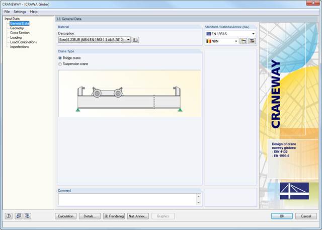
Geometry, material, cross-section, action, and imperfection data are entered in clearly arranged input windows:
Geometry
- Quick and convenient data input
- Definition of support conditions based on various support types (hinged, hinged movable, rigid, and user-defined, as well as lateral on upper or bottom flange)
- Optional specification of warping restraint
- Variable arrangement of rigid and deformable support stiffeners
- Possibility to insert hinges
CRANEWAY Cross-Sections
- I-shaped rolled cross-sections (I, IPE, IPEa, IPEo, IPEv, HE-B, HE-A, HE-AA, HL, HE-M, HE, HD, HP, IPB-S, IPB-SB, W, UB, UC, and other cross-sections according to AISC, ARBED, British Steel, Gost, TU, JIS, YB, GB, and others) combinable with section stiffener on the upper flange (angles or channels) as well as rail (SA, SF) or splice with user-defined dimensions
- Unsymmetrical I-sections (type IU) also combinable with stiffeners on the upper flange as well as with rail or splice
Actions
It is possible to consider the actions of up to three simultaneously operated cranes. You can simply select a standard crane from the library. You can also enter data manually:
- Number of cranes and crane axles (maximum of 20 axles per crane), center distances, position of crane buffers
- Classification in damage classes with editable dynamic factors according to EN 1993-6, and in lifting classes and exposure categories according to DIN 4132
- Vertical and horizontal wheel loads from self-weight, hoist load, mass forces from drive, as well as loads from skewing
- Axial loading in driving direction as well as buffer forces with user-defined eccentricities
- Permanent and variable secondary loads with user-defined eccentricities
Imperfections
- The imperfection load applies in compliance with the first natural vibration mode - either identically for all load combinations to be designed, or individually for each load combination, as mode shapes may vary depending on the load.
- Convenient tools available for scaling the mode shapes (rise determination of inclination and precamber).
Comprehensive and easy options in the individual input windows facilitate the representation of the structural system:
Nodal Supports
- The support type of each node is editable.
- It is possible to define a warp stiffening on each node. The resulting warp spring is determined automatically using the input parameters.
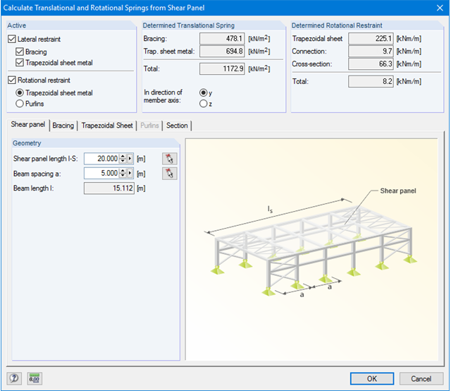
Elastic member foundation
- In the case of elastic member foundations, you can manually enter spring constants.
- Alternatively, you can use the various options to define the rotational and translational springs from a shear panel.
Member End Springs
- RF-/FE-LTB calculates the individual spring constants automatically. You can use the dialog boxes and detailed pictures to represent a translational spring by connecting component, a rotational spring by a connecting column, or a warping stiffener (available types: end plate, channel section, angle, connecting column, cantilevered portion).
Member Hinges
- If there are no member hinges defined in RFEM/RSTAB for the set of members, you can define them directly in the RF-/FE-LTB add-on module.
Load Data
- The nodal and member loads of the selected load cases and combinations are displayed in separate windows. There you can edit, delete, or add them individually.
Imperfections
- RF-/FE-LTB automatically applies the imperfections by scaling the lowest eigenvector.